Simultaneous Spatiotemporal Bias Compensation and Data Fusion for Asynchronous Multisensor Systems

Gongjian Zhou; Shizhe Bu; Thiagalingam Kirubarajan

doi:10.62762/CJIF.2024.361881

CiteScore

Impact Factor

Volume 1, Issue 1, Chinese Journal of Information Fusion

Volume 1, Issue 1, 2024

Submit Manuscript Edit a Special Issue

Table of Content

1. Introduction
2. Problem Formulation
3. Simultaneous Spatiotemporal Bias Compensation and Data Fusion
4. Lower Bound of Performance
5. Simulation Results
6. Conclusions

Chinese Journal of Information Fusion, Volume 1, Issue 1, 2024: 16-32

Open Access | Research Article | 27 May 2024

Simultaneous Spatiotemporal Bias Compensation and Data Fusion for Asynchronous Multisensor Systems

Gongjian Zhou 1 *

Shizhe Bu 1

Thiagalingam Kirubarajan 2

1 School of Electronics and Information Engineering, Harbin Institute of Technology, Harbin 150001, China

2 Department of Electrical and Computer Engineering, McMaster University, Ontario, Canada

* Corresponding Author: Gongjian Zhou, [email protected]

DOI: 10.62762/CJIF.2024.361881

Received: 17 February 2024, Accepted: 23 May 2024, Published: 27 May 2024

Cited by: 7 (Source: Web of Science) , 8 (Source: Google Scholar)

PDF (2.57 MB) Full-Text HTML XML

Article Metrics Cite This Article

Abstract

Bias estimation of sensors is an essential prerequisite for accurate data fusion. Neglect of temporal bias in general real systems prevents the existing algorithms from successful application. In this paper, both spatial and temporal biases in asynchronous multisensor systems are investigated and two novel methods for simultaneous spatiotemporal bias compensation and data fusion are presented. The general situation that the sensors sample at different times with different and varying periods is explored, and unknown time delays may exist between the time stamps and the true measurement times. Due to the time delays, the time stamp interval of the measurements from different sensors may be different from their true measurement interval, and the unknown difference between them is considered as the temporal bias and augmented into the state vector to be estimated. Multisensor measurements are collected in batch processing or sequential processing schemes to estimate the augmented state vector, results in two spatiotemporal bias compensation methods. In both processing schemes, the measurements are formulated as functions of both target states and spatiotemporal biases according to the time difference between the measurements and the states to be estimated. The Unscented Kalman Filter is used to handle the nonlinearity of the measurements and produce spatiotemporal bias and target state estimates simultaneously. The posterior Cramer-Rao lower bound (PCRLB) for spatiotemporal bias and state estimation is presented and simulations are conducted to demonstrate the effectiveness of the proposed methods.

Keywords

spatiotemporal bias

state estimation

multisensor data fusion

asynchronous sensors

1. Introduction

In a sensor network, data collected from multiple sensors [1, 3, 4, 8] is synergistically fused to improve overall system performance [2, 5, 6, 7]. An important prerequisite for successful fusion is that the spatial and temporal biases in asynchronous multiple sensor systems must be estimated and compensated. Otherwise, these biases may cause tracking performance degradation, and even worse, may lead to duplicate tracks.

Spatial bias estimation and compensation has been under intensive investigation for the past decades, and various algorithms have been developed in the literature. In [9], the real time quality control (RTQC) routine is developed to compute the bias by averaging the measurements from each sensor. In [10, 11, 12], the sensor registration is formulated as an ordinary or weighted least squares (LS) problem, and sensor biases are then estimated using LS technique. In [13], the exact maximum likelihood (EML) method is used to maximize the likelihood function of sensor measurements to obtain bias estimates. The method in [14] uses the maximum likelihood registration (MLR) method to solve the bias estimation problem of multiple dissimilar sensors. Another series of methods are based on filtering and use Kalman Filter (KF), extended Kalman Filter (EKF) and unscented Kalman Filter (UKF) to obtain online spatial bias estimates [15, 16, 17, 18, 19]. In [16], the KF method is used to estimate the sensor system bias and the attitude bias with the measurement noises being considered. In [17], the EKF method is used to estimate the position and azimuth biases of the distributed radars relative to the common reference coordinate system. Methods in [18, 19] use the augmented state Kalman filter (ASKF) to estimate the augmented state vectors including the target states and the biases of multisensor, so that the two components can be jointly estimated.

All these methods make one fundamental assumption, i.e., the time stamps of all the measurements accurately indicate the measurement times. In practical applications, there may be unknown time delays between them due to the latency of signal processing and/or data transfer. The time stamps cannot always be used as reliable time references to correctly fuse the measurements from multiple sensors, leading to temporal bias problems. The temporal bias must be accurately estimated and compensated, which is the focus of this paper.

Several algorithms have been developed to solve the temporal bias problem in offline mode. In [20, 21, 22], the temporal bias problem is considered in different combination of sensors. The time stamps and the unknown time delays are used to represent the true measurement times of sensors, and the measurement equations are formulated. The objective function of each sensor is built using the measurement error terms and the relevant covariances. The Levenberg-Marquardt (LM) algorithm [23] is used to find the ML estimates of the temporal bias and other unknown parameters based on minimizing the sum of objective functions. In [24], a generalized LS method is used to estimate the radar spatial bias and ADS-B temporal bias, where the radar has accurate time stamps while the transmitting time of ADS-B data packets are unavailable. The two sensors need to have same sampling period for this method to perform correctly. These methods [20, 21, 22, 24] do not consider the case where sensors all have unknown time delays. In [25], a multisensor time-offset estimation method is proposed for different time-offset statistical models and target dynamic models. This method assumes that the sensors are spatially unbiased and only estimates the temporal offset offline without compensation for accurate data fusion. These offline methods use the estimated bias as prior information to calibrate the sensors. This poses a problem that the bias may change each time the system is started, so the sensors have to be recalibrated.

In [26], an online method is proposed to estimate the temporal bias between the camera and the inertial measurement unit (IMU). The time stamps and the temporal bias estimates are used to represent the actual measurement times of the camera. However, due to temporal bias estimation errors, the camera measurements are inevitably processed at incorrect time instants, which may cause errors in the initial stage. Besides, the sensor spatial bias is not considered in this method. In [27, 28, 29], the spatial bias and the temporal bias are jointly considered for different combination of multiple dissimilar sensors. Three spatiotemporal bias estimation methods based on EKF, UKF and expectation-maximization-EKF (EM-EKF), respectively, are proposed to estimate the spatiotemporal biases and target states simultaneously. Since both biases may exist in practical multisensor systems, it is expected to jointly consider spatial and temporal biases into system models. In the three methods mentioned above, only the specific case where the multiple sensors have same sampling period is considered. In most real applications, the sensors may not sample at same time with same intervals.

In this paper, the problem of simultaneous spatiotemporal bias compensation and data fusion for practical multisensor systems, where the sampling periods of sensors may be different and varying, is investigated. In our previous papers [30, 31] on spatiotemporal bias estimation, the particular case where sensors have constant sampling periods is discussed. This paper is a significant extension of the previous work to the general case with varying sampling periods. We consider the difference between the time stamp interval and the true measurement interval of measurements from different sensors as the temporal bias, which is caused by the existence of unknown time delays. First, an augmented state equation combining the target state and spatiotemporal bias is formulated. Multisensor measurements are collected in batch processing or sequential processing schemes to estimate the augmented state vector, results in two spatiotemporal bias compensation methods. In batch processing scheme, multiple measurements from all sensors between two consecutive reference time instants are collected in a measurement vector to update the augmented state vector. We use the time stamp intervals and the temporal biases to represent the true measurement intervals, and an accurate relationship between measurements and states is established. In the sequential processing strategy, each measurement from each sensor is processed sequentially once available. Due to the unavailability of the true measurement intervals, the time stamp intervals are used to formulate state transition and the temporal bias is used to align the measurements with target states in measurement equations. In both processing schemes, the measurements are formulated as functions of both target states and spatiotemporal biases. This enables extraction of both spatial and temporal biases from the measurements. The UKF is used to handle the nonlinearity of the measurements to simultaneously estimate spatiotemporal biases and target states. The contributions of this paper can be summarized as follows:

The multisensor system with spatiotemporal bias is investigated and the time delay difference between the sensors is regarded as the temporal bias to be compensated for proper fusion of the measurements from the sensors.
The feasible state transitions are presented for the multisensor system without exactly known measurement interval.
The measurement equations are formulated to correctly describe the relationship between the measurements and the states with biased time.
Two spatiotemporal bias compensation methods are proposed to simultaneously estimate the biases and target states, one in batch processing scheme and the other in sequential processing scheme.
The posterior Cramer-Rao lower bound [32, 33] (PCRLB) is derived to quantify the best achievable performance.

The rest of the paper is organized as follows. In Section 2, the problem of spatiotemporal bias compensation and data fusion in asynchronous multisensor systems is formulated. In Section 3, the spatiotemporal bias compensation methods are presented in detail. The PCRLB of spatiotemporal bias and target state estimation is derived in Section 4. Section 5 presents the simulation results, followed by conclusions in Section 6.

2. Problem Formulation

Consider a centralized system with $N$ sensors that provides two-dimensional measurements in polar coordinates, namely range and azimuth measurements. The nearly constant velocity (NCV) motion model [34] of the target is considered in the whole paper. The target state vector is described as

X\left(k\right)={\left[{x\left(k\right),y\left(k\right),\dot{x}\left(k\right),% \dot{y}\left(k\right)}\right]^{\prime}}

where $x\left(k\right)$ and $y\left(k\right)$ are the positions in the direction of x and y, respectively, $\dot{x}\left(k\right)$ and $\dot{y}\left(k\right)$ are the corresponding velocities. Note that other target motion models can be handled seamlessly within the proposed methods. The target state equation is described as

\;X\left({k}\right)=F\left(k-1\right)\cdot X\left(k-1\right)+\Gamma\left(k-1% \right)\cdot v\left(k-1\right)

where $v\left(k-1\right)$ is the zero-mean Gaussian white process noise with known covariance $Q\left(k-1\right)$ , $F\left(k-1\right)$ is the state transition matrix, and $\Gamma\left(k-1\right)$ is the process noise gain matrix. The sensor $s$ reports range measurement $r_{s}\left(k\right)$ and azimuth measurement $\theta_{s}\left(k\right)$ at a rate, which may vary. The subscript $s$ denotes the sensor index and $k$ stands for the index of the measurement time ${t_{s}}\left(k\right)$ . The measurement equation is given by

\displaystyle\begin{array}[]{*{20}{l}}{z_{s}\left(k\right){\rm{=}}\;{h_{s}}% \left({k,X\left(k\right)}\right)+{w_{s}}\left(k\right)}\\ {\;\;\;\;\;\;\;\;\;=\left[{\begin{array}[]{*{20}{c}}{\displaystyle\sqrt{{{% \left({x\left(k\right)-x_{s}^{p}}\right)}^{2}}+{{\left({y\left(k\right)-y_{s}^% {p}}\right)}^{2}}}}\\ {\displaystyle\arctan\left({\displaystyle\frac{{y\left(k\right)-y_{s}^{p}}}{{x% \left(k\right)-x_{s}^{p}}}}\right)}\end{array}}\right]+{w_{s}}\left(k\right)}% \end{array}

where $\left({x_{s}^{p},\;y_{s}^{p}}\right)$ denotes the position of sensor $s$ , and ${w_{s}}\left(k\right)$ represents the zero-mean Gaussian white measurement noise with known covariance ${R_{s}}\left(k\right)$ , which is given as

{R_{s}}\left(k\right)={\rm{diag}}\left({\sigma_{r}^{2},\;\sigma_{\theta}^{2}}\right)

where $\sigma_{r}$ and $\sigma_{\theta}$ denote the standard deviations of range and azimuth measurement noises, respectively.

In practical systems, spatial bias ${b_{s}}={\left[{\Delta{r_{s}},\;\Delta{\theta_{s}}}\right]^{\prime}}$ of sensor $s$ may exist, where $\Delta{r_{s}}$ and $\Delta{\theta_{s}}$ stand for range bias and azimuth bias, respectively. Range bias may be caused by internal circuit delay in the sensor, zero drift in the system, or velocity incorrectness of the distance clock. Azimuth bias is usually caused by the deviation which appears when the sensor antenna is aligned with due North [35]. Additionally, the time stamps tagged to the measurements may be different from the true time that the target is observed. Normally, there may be time delays in the time stamps for a number of reasons. For example, some sensors take the time when the measurements are produced as the time stamps. Due to the latency of signal processing and/or data transfer, there is a time delay between the true measurement time and the generation of its time stamp. Different sensors may have different time delays due to different processing or communication latencies. If the time stamps are used as the true measurement times to perform time alignment for data fusion, large error and/or false correlation may be resulted, even there is no spatial bias. Therefore, in order to perform accurate data fusion, the spatiotemporal bias problem should be solved.

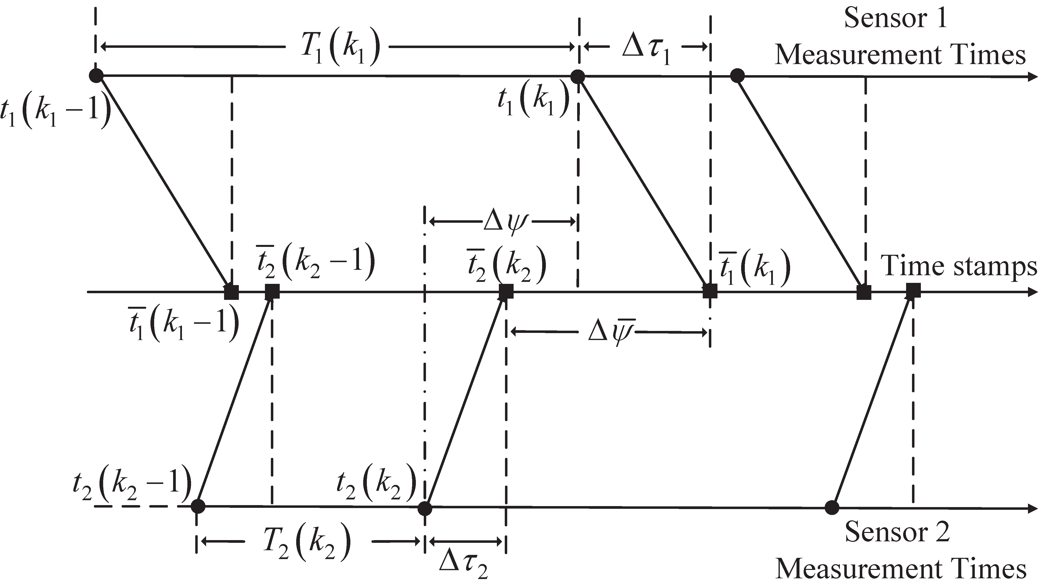
Figure 1 Time relationship among measurement times, time stamps and time delays.

3. Simultaneous Spatiotemporal Bias Compensation and Data Fusion

In this section, two spatiotemporal bias compensation methods are proposed for asynchronous multisensor systems. The general situation is considered, where sensors measure targets at different times with different and varying intervals. We take a two-sensor system as an example to present the time relationship among measurement times, time stamps and time delays, as illustrated in Figure 1.

In this figure, sensor $s=1,\;2$ measures target state with a varying period $T_{s}(k_{s})$ at the true measurement time $t_{s}(k_{s})$ , and the time stamp is ${\bar{t}_{s}}\left({{k_{s}}}\right)$ . Due to signal processing or communication latencies, there may exist unknown time delay $\Delta{\tau_{s}}={\bar{t}_{s}}\left({{k_{s}}}\right)-{t_{s}}\left({{k_{s}}}\right)$ between the time stamps of sensor $s$ with respect to the true measurement times. This prevents the time stamps from being used directly to perform proper time alignment and data fusion. For example, to fuse the $k_{1}\text{th}$ measurement from sensor 1 and the $k_{2}\text{th}$ measurement from sensor 2, the true measurement interval $\Delta\psi={t_{1}}\left({{k_{1}}}\right)-{t_{2}}\left({{k_{2}}}\right)$ between sensors is required. In practice, we only have the time stamp interval $\Delta\bar{\psi}={\bar{t}_{1}}\left({{k_{1}}}\right)-{\bar{t}_{2}}\left({{k_{2% }}}\right)$ . The temporal bias, $\Delta{t_{2,\;1}}=\Delta\bar{\psi}-\Delta\psi=\Delta{\tau_{1}}-\Delta{\tau_{2}}$ , between $\Delta\bar{\psi}$ and $\Delta\psi$ should be compensated for accurate data fusion. Note that we can only compensate for the temporal bias $\Delta{t_{2,\;1}}$ between the two sensors instead of the time delay of each sensor. Without loss of generality, we take sensor $1$ as the reference sensor and regard $\Delta{t_{s,\;1}}=\Delta{\tau_{1}}-\Delta{\tau_{s}},\;s=1,\ldots,N$ as relative temporal bias of sensor $s$ with respect to the reference sensor for the general case with $N$ sensors.

3.1 Augmented State Equation

In order to obtain effective data fusion in the presence of both spatial and temporal biases, the idea in this paper is to augment the spatiotemporal biases as a part of state vector to be estimated along with target states. The augmented state vector is given as

{\mathbf{X}}\left(k\right)=\left[{\begin{array}[]{*{20}{c}}{X\left(k\right)}\\ {{X^{b}}\left(k\right)}\end{array}}\right]

where ${{X}}\left(k\right)$ is the target base state vector, and ${X^{b}}\left(k\right)={\left[{B{{\left(k\right)}^{\prime}},\;\Psi{{\left(k% \right)}^{\prime}}}\right]^{\prime}}$ is the spatiotemporal biases of sensors. $B\left(k\right)$ consists of the spatial biases of $N$ sensors

B\left(k\right)=\left[{\begin{array}[]{*{20}{c}}{{b_{1}}\left(k\right)}\\ \vdots\\ {{b_{N}}\left(k\right)}\end{array}}\right]

and $\Psi\left(k\right)={\left[{\Delta{t_{2,\;1}}\left(k\right),\ldots,\;\Delta{t_{% N,\;1}}\left(k\right)}\right]^{\prime}}$ consists of the temporal biases of sensor $2,\ldots,N$ with respect to sensor 1.

Assume that the spatiotemporal biases provided by a sensor at different time instants are constants. The augmented state equation of (1) can be given by

{\bf{X}}\left({k}\right)={\bf{F}}\left(k-1\right)\cdot{\bf{X}}\left(k-1\right)% +{\bf{\Gamma}}\left(k-1\right)\cdot{{v}}\left(k-1\right)

where the augmented state transition matrix and the augmented process noise gain matrix are respectively given as

{\bf{F}}\left(k-1\right)=\left[{\begin{array}[]{*{20}{c}}{F\left(k-1\right)}&{% \bf{0}}_{4,\;(3N-1)}\\ {\bf{0}}_{(3N-1),\;4}&{{{\bf I}_{{\rm{3}}N-1}}}\end{array}}\right]

{\bf{\Gamma}}\left(k-1\right)=\left[{\begin{array}[]{*{20}{c}}{\Gamma\left(k-1% \right)}\\ {{{\bf{0}}_{\left({3N-1}\right),\;2}}}\end{array}}\right]

where ${{\bf{0}}_{{m},\;n}}$ denotes a ${{m}\cdot n}$ zero matrix, and ${{\bf I}_{{3N-1}}}$ denotes identity matrix of order ${{3N-1}}$ . Since the spatiotemporal biases are constants, there is no process noise with respect to the biases. The process noise $v(k-1)$ in (3) and its covariance are same to those of the process noise in (2). Assume the target moves according to the NCV model, the state transition matrix of the target base state is

F\left(k-1\right)=\left[{\begin{array}[]{*{20}{c}}1&0&{\Delta T\left(k-1\right% )}&0\\ 0&1&0&{\Delta T\left(k-1\right)}\\ 0&0&1&0\\ 0&0&0&1\end{array}}\right]

where $\Delta T\left(k-1\right)$ is the time interval between two consecutive states, which is considered in the filter. In the following, two measurement processing schemes, i.e., batch processing and sequential processing schemes, will be presented. Normally, the true measurement interval $\Delta\psi$ of two consecutive measurements should be used as the time interval $\Delta T\left(k-1\right)$ . Due to the existence of unknown time delays, the time stamp interval $\Delta\bar{\psi}$ instead of the true measurement interval $\Delta\psi$ is used to formulate the state transition.

In the batch processing scheme, we choose sensor $1$ as the reference sensor and update the state estimates using all the collected measurements when the measurements of sensor 1 are reported. Since the time delay of sensor 1 is constant, the measurement interval $\Delta\psi={t_{1}}\left(k\right)-{t_{1}}\left({k-1}\right)$ equals the time stamp interval $\Delta\bar{\psi}={{\bar{t}}_{1}}\left(k\right)-{{\bar{t}}_{1}}\left({k-1}\right)$ . We can use $\Delta\psi$ to exactly represent $\Delta T\left(k-1\right)$ .

In the sequential processing scheme, we estimate the augmented states once a measurement from one sensor is available, and the consecutive measurements may not originate from the same sensor. Since the time delays of sensors may be different, the true measurement interval $\Delta\psi$ is unavailable. In this case, the time stamp interval $\Delta\bar{\psi}$ instead of $\Delta\psi$ is used to formulate state transition. Assume two consecutive measurements are the $(k_{1}-1){\text{th}}$ and $(k_{2}-1){\text{th}}$ measurements from sensor 1 and sensor 2, respectively. One has

\begin{gathered}\Delta T\left({k-1}\right)=\Delta\bar{\psi}={{\bar{t}}_{2}}% \left({{k_{2}}-1}\right)-{{\bar{t}}_{1}}\left({{k_{1}}-1}\right)\hfill\\ \;\;\;\;\;\;\;\;\;\;\;\;\;\;\;\;\;\;=\Delta\psi+\Delta{t_{2,\;1}}\hfill\\ \end{gathered}

As shown in (7), temporal bias exists between $\Delta\bar{\psi}$ and $\Delta\psi$ , leading to bias in state transition. To eliminate this influence, the temporal bias is used in the measurement equation to align the measurements with target states.

3.2 The Measurement Equation

In practical multisensor systems, the sampling periods of multisensor may be different and varying. To handle the multisensor measurements in the general situation, two measurement processing scheme are presented. One is the batch processing scheme and the other is the sequential processing scheme. In the former, the sensor with longer sampling period is set as the reference sensor and multiple measurements from all sensors between two consecutive reference time instants are collected in a measurement vector to update the augmented state vector. For sequential processing scheme, each measurement from each sensor is processed sequentially to estimate the augmented state once it is available. For both schemes, the measurement equations are formulated as functions of the spatiotemporal biases and target base states, which enables simultaneous spatiotemporal bias estimation and data fusion.

3.2.1 Measurement Equation for Batch Processing Scheme

We consider the $k{\rm th}$ fusion period $\left({\left.{{{\bar{t}}_{1}}\left({k-1}\right),\;{{\bar{t}}_{1}}\left(k\right% )}\right]}\right.$ in this part, where ${\bar{t}_{1}}\left({k-1}\right)$ and ${\bar{t}_{1}}\left({k}\right)$ denote the time stamps of the $(k-1){\rm th}$ and $k{\rm th}$ measurements of sensor 1, which is chosen as the reference sensor. Let $m_{s}$ be the number of measurements provided by sensor $s$ in the current fusion period. The measurement vector ${\mathbb{Z}_{s}}\left(k\right)$ of sensor $s$ is given by

{\mathbb{Z}_{s}}\left(k\right)={\left[{z_{s}^{1}{{\left(k\right)}^{\prime}},% \ldots,z_{s}^{j}{{\left(k\right)}^{\prime}},\ldots,\;z_{s}^{{m_{s}}}{{\left(k% \right)}^{\prime}}}\right]^{\prime}}

where $z_{s}^{j}{\left(k\right)},\;j=1,\ldots,{m_{s}}$ denotes the $j{\text{th}}$ measurement provided by sensor $s$ in the $k{\text{th}}$ fusion period and its time stamp $\bar{t}_{s}^{j}\left(k\right)$ falls within the period $\left({\left.{{{\bar{t}}_{1}}\left({k-1}\right),\;{{\bar{t}}_{1}}\left(k\right% )}\right]}\right.$ . The measurement vector $\mathbb{Z}\left(k\right)$ of all sensors in the current fusion period is given by

\mathbb{Z}\left(k\right)={\left[{{\mathbb{Z}_{1}}{{\left(k\right)}^{\prime}},% \;{\mathbb{Z}_{2}}{{\left(k\right)}^{\prime}},\ldots,\;{\mathbb{Z}_{N}}{{\left% (k\right)}^{\prime}}}\right]^{\prime}}.

As discussed in Section 3.1, the time interval $\Delta T(k-1)$ in state transition matrix equals the true measurement interval. Therefore, the augmented state estimate is updated at the measurement time $t_{1}(k)$ of sensor 1 using the measurement vector $\mathbb{Z}\left(k\right)$ . To properly formulate the measurement equation, the true interval between measurement time $t_{1}(k)$ and measurement time $t_{s}^{j}\left(k\right)$ , $\Delta\psi_{s}^{j}={t_{1}}\left(k\right)-t_{s}^{j}\left(k\right)$ , is required for alignment of the measurements from sensors with the state to be updated. However, we only have the time stamp interval $\Delta\bar{\psi}_{s}^{j}={\bar{t}_{1}}\left(k\right)-{\bar{t}_{s}^{j}}\left({k% }\right)$ , where unknown temporal bias $\Delta{t_{s,\;1}}=\Delta\bar{\psi}_{s}^{j}-\Delta\psi_{s}^{j}$ between $\Delta\bar{\psi}_{s}^{j}$ and $\Delta\psi_{s}^{j}$ exists. Here, the solution is to use $\Delta\bar{\psi}_{s}^{j}-\Delta{t_{s,\;1}}$ to replace $\Delta\psi_{s}^{j}$ in the measurement equation. Since $\Delta{t_{s,\;1}}$ is part of the augmented state vector, this replacement enables exact description of the relationship between the measurements in (9) and the augmented states in (1).

Here, we denote $\Delta{t_{s,\;1}}=0,\;s=1$ as the temporal bias of sensor 1 relative to itself, which is used to ensure that the measurement equation of sensor 1 can be formulated using the general expression, just like other sensors. The measurements in (9) are formulated as functions of the target states, spatiotemporal biases and the time stamp intervals

\begin{array}[]{*{20}{l}}{z\left(k\right)=h\left({{\mathbf{X}}\left(k\right)}% \right)+{\mathbf{w}}\left(k\right)}\\ {\;\;\;\;\;\;\;\;={{\left[{{h_{1}}{{\left({{\mathbf{X}}\left(k\right)}\right)}% ^{\prime}},\ldots,\;{h_{N}}{{\left({{\mathbf{X}}\left(k\right)}\right)}^{% \prime}}}\right]}^{\prime}}+{\mathbf{w}}\left(k\right)}\end{array}

where ${h_{s}}\left({{\mathbf{X}}\left(k\right)}\right),\;s=1,\ldots,\;N$ denotes the measurement function of sensor $s$ , ${\mathbf{w}}\left(k\right)$ denotes the zero-mean Gaussian white measurement noise with known covariance $\Re\left(k\right)$ , which is given by

\Re\left(k\right)={\text{diag}}\left({{{\mathbf{R}}_{1}}\left(k\right),\ldots,% {{\mathbf{R}}_{s}}\left(k\right),\ldots,{{\mathbf{R}}_{N}}\left(k\right)}\right)

where

{{\mathbf{R}}_{s}}\left(k\right)={\text{diag}}\left({R_{s}^{1}\left(k\right),% \ldots,R_{s}^{j}\left(k\right),\ldots,R_{s}^{{m_{s}}}\left(k\right)}\right)

and $R_{s}^{j}\left(k\right)={\rm{diag}}\left({\sigma_{r}^{2},\;\sigma_{\theta}^{2}% }\right)$ . The measurement function ${h_{s}}\left({{\mathbf{X}}\left(k\right)}\right)$ of sensor $s$ is

\begin{array}[]{l}{h_{s}}\left({{\mathbf{X}}\left(k\right)}\right)=\\ \left[{\begin{array}[]{*{20}{c}}{\sqrt{{{\left({x_{s}^{1}\left(k\right)-x_{s}^% {p}}\right)}^{2}}+{{\left({y_{s}^{1}\left(k\right)-y_{s}^{p}}\right)}^{2}}}+% \Delta{r_{s}}\left(k\right)}\\ {\displaystyle\arctan\left({\frac{{y_{s}^{1}\left(k\right)-y_{s}^{p}}}{{x_{s}^% {1}\left(k\right)-x_{s}^{p}}}}\right)+\Delta{\theta_{s}}\left(k\right)}\\ \vdots\\ {\sqrt{{{\left({x_{s}^{j}\left(k\right)-x_{s}^{p}}\right)}^{2}}+{{\left({y_{s}% ^{j}\left(k\right)-y_{s}^{p}}\right)}^{2}}}+\Delta{r_{s}}\left(k\right)}\\ {\displaystyle\arctan\left({\frac{{y_{s}^{j}\left(k\right)-y_{s}^{p}}}{{x_{s}^% {j}\left(k\right)-x_{s}^{p}}}}\right)+\Delta{\theta_{s}}\left(k\right)}\\ \vdots\\ {\sqrt{{{\left({x_{s}^{{m_{s}}}\left(k\right)-x_{s}^{p}}\right)}^{2}}+{{\left(% {y_{s}^{{m_{s}}}\left(k\right)-y_{s}^{p}}\right)}^{2}}}+\Delta{r_{s}}\left(k% \right)}\\ {\displaystyle\arctan\left({\frac{{y_{s}^{{m_{s}}}\left(k\right)-y_{s}^{p}}}{{% x_{s}^{{m_{s}}}\left(k\right)-x_{s}^{p}}}}\right)+\Delta{\theta_{s}}\left(k% \right)}\end{array}}\right]\end{array}

with

\left\{{\begin{array}[]{*{20}{c}}{\begin{array}[]{*{20}{c}}{x_{s}^{j}\left(k% \right)=x\left(k\right)-\dot{x}\left(k\right)\cdot\left({\Delta\bar{\psi}_{s}^% {j}-\Delta{t_{s,\;1}}(k)}\right)}\\ {y_{s}^{j}\left(k\right)=y\left(k\right)-\dot{y}\left(k\right)\cdot\left({% \Delta\bar{\psi}_{s}^{j}-\Delta{t_{s,\;1}}(k)}\right)}\end{array}}\\ {\Delta\bar{\psi}_{s}^{j}={{\bar{t}}_{1}}\left(k\right)-\bar{t}_{s}^{j}\left(k% \right)}\end{array}}\right.

where $\left({x_{s}^{p},\;y_{s}^{p}}\right)$ denotes the position of sensor $s$ , $\Delta{r_{s}}\left(k\right)$ and $\Delta{\theta_{s}}\left(k\right)$ denote the range and azimuth biases of sensor $s$ , respectively, and $\left({{x_{s}^{j}}\left(k\right),\;{y_{s}^{j}}\left(k\right)}\right),\;s=1,% \ldots,N,\;j=1,\ldots,{m_{s}}$ denotes the true target position corresponding to the measurement $z_{s}^{j}(k)$ at time $t_{s}^{j}(k)$ . We use ${\Delta\bar{\psi}_{s}^{j}-\Delta{t_{s,\;1}}}$ to represent the true measurement interval between the time $t_{1}(k)$ and the measurement time $t_{s}^{j}(k)$ , which enables each measurement of sensor $s$ to be correctly represented by the target states, spatiotemporal biases and the time stamp intervals according to (13). As a result, the spatiotemporal biases and target states can be estimated simultaneously from the measurements collected in (9).

3.2.2 Measurement Equation for Sequential Processing Scheme

In this part, the measurement equation for sequential processing scheme is presented. We denote ${t_{s}}\left({{k_{s}}}\right)$ and ${\bar{t}_{s}}\left({{k_{s}}}\right)$ as the true measurement time and the time stamp, respectively, corresponding to the ${k_{s}}{\text{th}}$ measurement $z_{s}(k_{s})$ from sensor $s$ . The sensor that first provides a measurement is chosen as the reference sensor. Without loss of generality, we assume sensor $1$ is the reference sensor and denote $\Delta{t_{s,\;1}}=0,\;s=1$ as the temporal bias of sensor $1$ relative to itself. To avoid ambiguity, we denote $k$ as the overall measurement index across all sensors. Each time a measurement is received at the fusion center, $k$ is incremented by 1. The example given in Figure 1 is used to illustrate the formulation of the measurement equation, followed by the general case with $N$ sensors.

Assume that the $({k_{1}-1}){\text{th}}$ measurement $z_{1}(k_{1}-1)$ provided by sensor $1$ is the $({k-1}){\text{th}}$ measurement received at the fusion center. We use $z_{1}(k_{1}-1)$ to initialize the augmented state at time $t_{1}(k_{1}-1)$ , as will be presented in Section 3.4. As shown in Figure 1, the consecutive measurements may be from the same sensor or different sensors, and there are four possible combinations of their sources. The measurement equations for all the four cases are formulated as follows.

The previous measurement $z_{1}(k_{1}-1)$ with the overall measurement index $k-1$ and the current measurement ${z_{2}}\left({{k_{2}-1}}\right)$ with the overall measurement index $k$ are from sensor 1 and sensor 2, respectively: In this case, the true measurement interval $\Delta\psi={t_{2}}\left({{k_{2}}-1}\right)-{t_{1}}\left({{k_{1}}-1}\right)$ between ${z_{2}}\left({{k_{2}-1}}\right)$ and ${z_{1}}\left({{k_{1}-1}}\right)$ is unavailable since their time stamp delays may be different. As discussed in Section 3.1, we use the time stamp interval $\Delta\bar{\psi}={\bar{t}_{2}}\left({{k_{2}}-1}\right)-{\bar{t}_{1}}\left({{k_% {1}}-1}\right)$ instead of $\Delta\psi$ to represent the time interval $\Delta T\left({k-1}\right)$ in the state transition matrix. After transition according to $\Delta\bar{\psi}$ , the true time of the state ${\mathbf{X}}\left(k\right)$ is ${t_{2}}\left(k_{2}-1\right)-\Delta{t_{2,\;1}}$ and unequal to the measurement time ${t_{2}}\left(k_{2}-1\right)$ . To eliminate this influence, the temporal bias is used to align the measurement with the state ${\mathbf{X}}\left(k\right)$ in measurement equation, as given by

\begin{gathered}z\left(k\right)=h\left({{\mathbf{X}}\left(k\right)}\right)+{w_% {s}}\left(k\right)\hfill\\ \;\;\;\;\;\;\;=\left[{\begin{array}[]{*{20}{c}}{\sqrt{{x_{s}}{{\left(k\right)}% ^{2}}+{y_{s}}{{\left(k\right)}^{2}}}+\Delta{r_{s}}\left(k\right)}\\ {\displaystyle\arctan\left({\frac{{{y_{s}}\left(k\right)}}{{{x_{s}}\left(k% \right)}}}\right)+\Delta{\theta_{s}}\left(k\right)}\end{array}}\right]+{w_{s}}% \left(k\right)\hfill\\ \end{gathered}

\left\{{\begin{array}[]{*{20}{c}}{{x_{s}}\left(k\right)=x\left(k\right)+\dot{x% }\left(k\right)\cdot\Delta{t_{s,\;1}}\left(k\right)-x_{s}^{p}}\\ {{y_{s}}\left(k\right)=y\left(k\right)+\dot{y}\left(k\right)\cdot\Delta{t_{s,% \;1}}\left(k\right)-y_{s}^{p}}\end{array}}\right.

where $s=2$ , $\left({x_{s}^{p},\;y_{s}^{p}}\right)$ denotes the position of sensor $s$ , ${w_{s}}\left(k\right)$ denotes the zero-mean Gaussian white measurement noise with known covariance $\Re\left(k\right)={\rm{diag}}\left({\sigma_{r}^{2},\;\sigma_{\theta}^{2}}\right)$ , and $\left({{x_{s}}\left(k\right),\;{y_{s}}\left(k\right)}\right)$ denotes the true target position corresponding to the measurement ${z_{2}}\left({{k_{2}-1}}\right)$ at time $t_{2}(k_{2}-1)$ . We utilize $\Delta{t_{s,\;1}}$ to represent the true interval between the time ${t_{2}}\left(k_{2}-1\right)-\Delta{t_{2,\;1}}$ of the state ${\mathbf{X}}\left(k\right)$ and the measurement time ${t_{2}}\left(k_{2}-1\right)$ , which enables each measurement of sensor $s$ to be correctly represented by the target states and spatiotemporal biases according to (15a). Accordingly, the spatiotemporal biases and target states can be estimated simultaneously using the measurement from sensor $s$ .

b) Both the previous measurement ${z_{2}}\left({{k_{2}-1}}\right)$ with the overall measurement index $k$ and the current measurement ${z_{2}}\left({{k_{2}}}\right)$ with the overall measurement index $k+1$ are from sensor 2: In this case, the measurement interval $\Delta\psi$ equals the time stamp interval $\Delta\bar{\psi}$ since the time delay of sensor 2 is constant. One has

\Delta T\left(k\right)=\Delta\bar{\psi}={\bar{t}_{2}}\left({{k_{2}}}\right)-{% \bar{t}_{2}}\left({{k_{2}}-1}\right)=\Delta\psi.

After state transition from the previous update time ${t_{2}}\left(k_{2}-1\right)-\Delta{t_{2,\;1}}$ according to $\Delta T\left({k}\right)$ , the time of the state is ${t_{2}}\left({{k_{2}}}\right)-\Delta{t_{2,\;1}}$ , which is still unequal to the measurement time of $z_{2}(k_{2})$ . This influence can be eliminated in the similar way as in Section 3.2.2, and the measurement equation can be formulated in the same way as in (15) except that the overall measurement index is $k+1$ .

c) The previous measurement ${z_{2}}\left({{k_{2}}}\right)$ with the overall measurement index $k+1$ and the current measurement ${z_{1}}\left({{k_{1}}}\right)$ with the overall measurement index $k+2$ are from sensor 2 and sensor 1, respectively: In this case, the time interval $\Delta T\left(k+1\right)$ is

\begin{gathered}\Delta T\left(k+1\right)=\Delta\bar{\psi}={{\bar{t}}_{1}}\left% ({{k_{1}}}\right)-{{\bar{t}}_{2}}\left({{k_{2}}}\right)\hfill\\ \;\;\;\;\;\;\;\;\;\;\;\;\;\;\;\;\;\;=\Delta\psi+\Delta{t_{2,\;1}}\hfill\\ \end{gathered}.

After state transition from the previous update time ${t_{2}}\left(k_{2}\right)-\Delta{t_{2,\;1}}$ according to $\Delta T\left({k+1}\right)$ , the time of the state is ${t_{1}}\left({{k_{1}}}\right)$ and equals the measurement time of $z_{1}(k_{1})$ . We have denoted the temporal bias of sensor $1$ relative to itself as $\Delta{t_{1,\;1}}=0$ , so the measurement equation of sensor 1 can be formulated using the general expression (15) except that the overall measurement index is $k+2$ and the sensor index $s$ is 1.

d) Both the previous measurement ${z_{1}}\left({{k_{1}}}\right)$ with the overall measurement index $k+2$ and the current measurement ${z_{1}}\left({{k_{1}+1}}\right)$ with the overall measurement index $k+3$ are from sensor 1: In this case, the time interval $\Delta T\left({k+2}\right)$ equals the true measurement interval $\Delta\psi$ . After state transition from the previous update time ${t_{1}}\left(k_{1}\right)$ according to $\Delta T\left({k+2}\right)$ , the time of the state is ${t_{1}}\left({{k_{1}+1}}\right)$ and equals the measurement time of $z_{1}(k_{1}+1)$ . The measurement equation can be formulated in the same way as in (15) except that the overall measurement index is $k+3$ and the sensor index $s$ is 1.

The above cases encompass all possible combinations of the sources for consecutive measurements, without other possibilities. When the subsequent measurements are received at the fusion center, the measurement equations can be formulated according to one of the cases.

Referring to the above formulation in the case with two sensors, the general expression for the measurement equation can be formulated for a system with $N$ sensors. We denote ${\bar{t}_{{p}}}\left({{k_{{p}}}}\right)$ and ${\bar{t}_{{c}}}\left({{k_{{c}}}}\right)$ as the time stamps when the previous and current measurements are provided by sensor $p$ and $c$ , respectively, where $p,\;c=1,\ldots,N$ . When the current measurement ${z_{c}}\left({{k_{c}}}\right)$ with overall measurement index $k$ is received at the fusion center, the time interval is $\Delta T\left(k-1\right)={\bar{t}_{{c}}}\left({{k_{{c}}}}\right)-{\bar{t}_{{p}% }}\left({{k_{{p}}}}\right)$ . Substituting $\Delta T\left(k-1\right)$ into (6), we can formulate the corresponding transition matrix, and the augmented state equation is formulated according to (3) $-$ (5). The expression for the measurement equation is the same as (15) except that the subscript $s$ needs to be replaced by subscript $c$ .

3.3 Filtering Process

Owing to the nonlinearity of the measurement equations in Section 3.2, the Unscented Kalman Filter (UKF) is employed to jointly estimate the spatiotemporal biases and target states. This leads to two approaches: batch processing-based (BP-SBDF) and sequential processing-based (SP-SBDF) spatiotemporal bias compensation and data fusion.

The UKF uses the unscented transformation [36] (UT) to approximate the mean and covariance of the augmented state and measurement. First, the sigma points $\delta$ and the associated weights $W$ are calculated given the augmented state estimate ${\bf{\hat{X}}}\left({k-1\left|{k-1}\right.}\right)$ and state estimation covariance ${\bf{P}}\left({k-1\left|{k-1}\right.}\right)$ . The mean and covariance are then approximated by using a weighted sample mean and covariance of these sigma points. That is

\left\{\begin{array}[]{l}{\delta_{i}}\left({k-1\left|{k-1}\right.}\right)={\bf% {\hat{X}}}\left({k-1\left|{k-1}\right.}\right),\\ \;\;\;\;\;\;\;\;\;\;\;\;\;\;\;\;\;\;\;\;{W_{0}}=\displaystyle\frac{\kappa}{{{n% _{x}}+\kappa}},\;\;\;\;\;\;i=0\;;\\ {\delta_{i}}\left({k-1\left|{k-1}\right.}\right)={\bf{\hat{X}}}\left({k-1\left% |{k-1}\right.}\right)\\ \;\;\;\;\;\;\;\;\;\;\;\;\;\;\;\;\;\;\;\;\;\;\;\;\;\;\;\;\;+{\left({\sqrt{\left% ({{n_{x}}+\kappa}\right){\bf{P}}\left({k-1\left|{k-1}\right.}\right)}}\right)_% {i}},\\ \;\;\;\;\;\;\;\;\;\;\;\;\;\;\;\;\;\;\;{W_{i}}=\displaystyle\frac{1}{{2({n_{x}}% +\kappa)}},\;\;i=1,\cdots,{n_{x}}\;;\\ {\delta_{i}}\left({k-1\left|{k-1}\right.}\right)={\bf{\hat{X}}}\left({k-1\left% |{k-1}\right.}\right)\\ \;\;\;\;\;\;\;\;\;\;\;\;\;\;\;\;\;\;\;\;\;\;\;\;\;\;\;\;\;-{\left({\sqrt{\left% ({{n_{x}}+\kappa}\right){\bf{P}}\left({k-1\left|{k-1}\right.}\right)}}\right)_% {i}},\\ \;\;\;\;\;\;\;\;\;\;\;\;\;\;\;\;\;\;\;{W_{i}}=\displaystyle\frac{1}{{2({n_{x}}% +\kappa)}},\;\;i={n_{x}}+1,\cdots,2{n_{x}}\;;\end{array}\right.

where $n_{x}$ is the dimension of the augmented state, ${\delta_{i}}\left({k-1\left|{k-1}\right.}\right)$ is the $i$ th sigma point, ${W_{i}}$ is the associated weight, $\kappa$ is the scale parameter, and ${\left({\sqrt{\left({n_{x}+\kappa}\right){\bf P}\left({k-1\left|{k-1}\right.}% \right)}}\right)_{i}}$ is the $i$ th row or column of the matrix square root.

These sigma points can be updated using the augmented state equation given by (3)

\begin{array}[]{l}{\delta_{i}}\left({k\left|{k-1}\right.}\right)={\bf{F}}\left% ({k-1}\right)\cdot{\delta_{i}}\left({k-1\left|{k-1}\right.}\right),\\ \;\;\;\;\;\;\;\;\;\;\;\;\;\;\;\;\;\;\;\;\;\;\;\;\;\;\;\;\;\;\;\;\;i=1,\cdots,2% {n_{x}}\;.\end{array}

The weighted mean of these predicted sigma points for the augmented state is given by

\hat{\bf{X}}\left({k\left|k-1\right.}\right)=\sum\limits_{i=0}^{2n_{x}}{{W_{i}% }\cdot{\delta_{i}}\left({k\left|k-1\right.}\right)}\;.

The prediction covariance of the augmented state is calculated by

\begin{array}[]{l}{\bf{P}}\left({k\left|{k-1}\right.}\right)=\sum\limits_{i=0}% ^{2{n_{x}}}{{W_{i}}\cdot\Delta{{\bf{X}}_{i}}\left({k\left|{k-1}\right.}\right)% }\cdot{\left({\Delta{{\bf{X}}_{i}}\left({k\left|{k-1}\right.}\right)}\right)^{% \prime}}\\ \;\;\;\;\;\;\;\;\;\;\;\;\;\;\;\;\;\;\;\;\;\;\;+\;Q\left({k-1}\right)\end{array}

where

\Delta{{\bf{X}}_{i}}\left({k\left|k-1\right.}\right)={\delta_{i}}\left({k\left% |k-1\right.}\right)-\hat{\bf{X}}\left({k\left|k-1\right.}\right)

and $Q\left(k-1\right)$ denotes the known process noise covariance. We denote ${\eta_{i}}\left({k\left|k-1\right.}\right)$ as the prediction of sigma points for the measurements. Note that the measurement equations for BP-SBDF method and SP-SBDF method are different, and their expressions have been given by (10) and (15), respectively. Substituting ${{\delta_{i}}\left({k\left|k-1\right.}\right)}$ into the corresponding measurement functions, we have

{\eta_{i}}\left({k\left|k-1\right.}\right)=h\left({{\delta_{i}}\left({k\left|k% -1\right.}\right)}\right)\;.

The weighted mean of these sigma points for the measurement is given by

\hat{z}\left({k\left|k-1\right.}\right)=\sum\limits_{i=0}^{2{n_{x}}}{{W_{i}}% \cdot{\eta_{i}}\left({k\left|k-1\right.}\right)}\;.

The covariance of the predicted measurement is given by

\begin{array}[]{l}\begin{aligned} {{\mathbf{P}}_{zz}}\left({k}\right)=&\sum% \limits_{i=0}^{2{n_{x}}}{{W_{i}}\cdot\Delta{z_{i}}\left({k\left|k-1\right.}% \right)}\cdot{\left({\Delta{z_{i}}\left({k\left|k-1\right.}\right)}\right)^{% \prime}}\\ &+\Re\left({k}\right)\;\end{aligned}\end{array}

where

\Delta{z_{i}}\left({k\left|k-1\right.}\right)={\eta_{i}}\left({k\left|k-1% \right.}\right)-\hat{z}\left({k\left|k-1\right.}\right)

and $\Re\left({k}\right)$ denotes the known measurement noise covariance and has two different expressions in BP-SBDF and SP-SBDF methods. The cross-covariance between the augmented states and measurements is given by

{{\bf{P}}_{xz}}\left(k\right)=\sum\limits_{i=0}^{2{n_{x}}}{{W_{i}}\cdot\Delta{% {\bf{X}}_{i}}\left({k\left|k-1\right.}\right)\cdot{{\left({\Delta{z_{i}}\left(% {k\left|k-1\right.}\right)}\right)}^{\prime}}}\;.

The filter gain can then be given by

K\left({k}\right)={{\bf{P}}_{xz}}\left({k}\right){{\bf{P}}_{zz}}{\left({k}% \right)^{-1}}\;.

Finally, the augmented state estimate and the corresponding covariance are updated by

{\bf{\hat{X}}}\left({k\left|{k}\right.}\right)={\bf{\hat{X}}}\left({k\left|k-1% \right.}\right)+K\left({k}\right)\cdot\left({z\left({k}\right)-\hat{z}\left({k% \left|k-1\right.}\right)}\right)

and

{\bf P}\left({k\left|{k}\right.}\right)={\bf P}\left({k\left|k-1\right.}\right% )-K\left({k}\right){{\bf{P}}_{zz}}\left({k}\right)K^{\prime}\left({k}\right)\;.

3.4 Filter Initialization

In this subsection, the one-point initialization method [37] is used to estimate the initial augmented state and its covariance for the two proposed methods. The basic idea is to estimate initial target state using the first reported measurement and find the initial covariance by the measurement covariance. Without loss of generality, we assume sensor $1$ first provides the measurement $z_{1}(1)$ in polar coordinates. The unbiased conversion from polar coordinates to Cartesian coordinates [38, 39, 40] can be given by

z_{1}^{u}\left(1\right)=\left[{\begin{array}[]{*{20}{c}}{x_{1}^{u}\left(1% \right)}\\ {y_{1}^{u}\left(1\right)}\end{array}}\right]=\left[{\begin{array}[]{*{20}{c}}{% \lambda_{\theta}^{-1}{r_{1}}\left(1\right)\cos\left({{\theta_{1}}\left(1\right% )}\right)}\\ {\lambda_{\theta}^{-1}{r_{1}}\left(1\right)\sin\left({{\theta_{1}}\left(1% \right)}\right)}\end{array}}\right]-{\mu^{u}}

where ${x_{1}^{u}\left(1\right)}$ and ${y_{1}^{u}\left(1\right)}$ are the unbiased converted measurements in x and y directions, respectively, ${r_{1}}\left(1\right)$ and ${\theta_{1}}\left(1\right)$ are the first range and azimuth measurements reported by sensor 1, respectively. $\lambda_{\theta}$ is the bias compensation factor, and ${\mu^{u}}$ is the mean of the converted measurement error, which are respectively given by

{\lambda_{\theta}}={e^{{{-\sigma_{\theta}^{2}}\mathord{\left/{\vphantom{{-% \sigma_{\theta}^{2}}2}}\right.\kern-1.2pt}2}}}

{\mu^{u}}=\left[{\begin{array}[]{*{20}{c}}{\left({\lambda_{\theta}^{-1}-{% \lambda_{\theta}}}\right){r_{1}}\left(1\right)\cos\left({{\theta_{1}}\left(1% \right)}\right)}\\ {\left({\lambda_{\theta}^{-1}-{\lambda_{\theta}}}\right){r_{1}}\left(1\right)% \sin\left({{\theta_{1}}\left(1\right)}\right)}\end{array}}\right].

The converted measurement covariance $R_{1}^{u}\left(1\right)$ is

R_{1}^{u}\left(1\right)=\left[{\begin{array}[]{*{20}{c}}{R_{1}^{u,\;11}\left(1% \right)}&{R_{1}^{u,\;12}\left(1\right)}\\ {R_{1}^{u,\;21}\left(1\right)}&{R_{1}^{u,\;22}\left(1\right)}\end{array}}\right]

where

\begin{gathered}R_{1}^{u,\;11}\left(1\right)=-\lambda_{\theta}^{2}r_{1}^{2}% \left(1\right){\cos^{2}}\left({{\theta_{1}}\left(1\right)}\right)\hfill\\ \;\;\;\;\;\;\;\;\;\;\;\;+\frac{1}{2}\left({r_{1}^{2}\left(1\right)+\sigma_{r}^% {2}}\right)\left({1+{\alpha_{\theta}}\cos\left({2{\theta_{1}}\left(1\right)}% \right)}\right)\hfill\\ \end{gathered}

\begin{gathered}R_{1}^{u,\;22}\left(1\right)=-\lambda_{\theta}^{2}r_{1}^{2}% \left(1\right){\sin^{2}}\left({{\theta_{1}}\left(1\right)}\right)\hfill\\ \;\;\;\;\;\;\;\;\;\;\;\;+\frac{1}{2}\left({r_{1}^{2}\left(1\right)+\sigma_{r}^% {2}}\right)\left({1-{\alpha_{\theta}}\cos\left({2{\theta_{1}}\left(1\right)}% \right)}\right)\hfill\\ \end{gathered}

\begin{gathered}R_{1}^{u,\;12}\left(1\right)=R_{1}^{u,\;21}{\left(1\right)}=-% \lambda_{\theta}^{2}r_{1}^{2}\left(1\right)\sin\left({{\theta_{1}}\left(1% \right)}\right)\cos\left({{\theta_{1}}\left(1\right)}\right)\hfill\\ \;\;\;\;\;\;\;\;\;\;\;\;+\frac{1}{2}\left({r_{1}^{2}\left(1\right)+\sigma_{r}^% {2}}\right){\alpha_{\theta}}\sin\left({2{\theta_{1}}\left(1\right)}\right)% \hfill\\ \end{gathered}

and ${\alpha_{\theta}}={e^{-2\sigma_{\theta}^{2}}}$ . Based on one position measurement, one has no information on target velocity. If the maximum target velocity is $v_{\text{max}}$ , the uniform distribution of target velocity with appropriate bounds may reflect our ignorance. This uniform distribution is replaced by a Gaussian probability distribution function with mean zero and covariance ${v_{\max}^{2}\cdot{{\bf I}_{2}}}/3$ for velocity. The initial estimate of the target state and its covariance are respectively given by

\hat{X}\left({1\left|1\right.}\right)={\left[{\begin{array}[]{*{20}{c}}{x_{1}^% {u}\left(1\right)}&{y_{1}^{u}\left(1\right)}&0&0\end{array}}\right]^{\prime}}

P\left({1\left|1\right.}\right)=\left[{\begin{array}[]{*{20}{c}}R_{1}^{u}\left% (1\right)&{{{\bf{0}}_{2,\;2}}}\\ {{{\bf{0}}_{2,\;2}}}&{{v_{\max}^{2}\cdot{{\bf I}_{2}}}/3}\end{array}}\right]

where ${{{\bf{0}}_{2,\;2}}}$ is a $2\cdot 2$ zero matrix, and ${{\bf I}_{2}}$ is a identity matrix with order 2.

There is no prior information about the spatial and temporal biases, and we set their initial estimates to zero, that is, ${\hat{X}^{b}}\left({1\left|1\right.}\right)={{\mathbf{0}}_{\left({3N-1}\right)% ,\;1}}$ . Additionally, we assume the target states and the spatiotemporal biases are uncorrelated, and the independent bias assumption results in block diagonal covariance matrices of the spatiotemporal biases. As in (39), the maximum range and azimuth biases are assumed to be $\Delta{r_{\max}}$ and $\Delta{\theta_{\max}}$ , respectively, and the maximum temporal bias is $\Delta{t_{\max}}$ . The initial estimate of the covariance for spatiotemporal biases is

{P^{b}}\left({1\left|1\right.}\right)={\text{diag}}\left({\underbrace{P_{B}^{b% },\ldots\;,P_{B}^{b}}_{N},\underbrace{P_{\Psi}^{b},\ldots\;,P_{\Psi}^{b}}_{N-1% }}\right)

where

\left\{{\begin{array}[]{*{20}{c}}{P_{B}^{b}={\rm{diag}}\left({{{\Delta r_{\max% }^{2}}\mathord{\left/{\vphantom{{\Delta r_{\max}^{2}}3}}\right.\kern-1.2pt}3},% \;{{\Delta\theta_{\max}^{2}}\mathord{\left/{\vphantom{{\Delta\theta_{\max}^{2}% }3}}\right.\kern-1.2pt}3}}\right)}\\ {P_{\Psi}^{b}={{\Delta t_{\max}^{2}}\mathord{\left/{\vphantom{{\Delta t_{\max}% ^{2}}3}}\right.\kern-1.2pt}3}}\end{array}}\right..

As a result, the initial estimates of the augmented state and its covariance are

{\mathbf{\hat{X}}}\left({1\left|1\right.}\right)=\left[{\begin{array}[]{*{20}{% c}}{\hat{X}\left({1\left|1\right.}\right)}\\ {{{\hat{X}}^{b}}\left({1\left|1\right.}\right)}\end{array}}\right]

and

{\mathbf{P}}\left({1\left|1\right.}\right)={\text{diag}}\left({P\left({1\left|% 1\right.}\right),\;{P^{b}}\left({1\left|1\right.}\right)}\right).

4. Lower Bound of Performance

Since the measurement equations are nonlinear, the optimal solution to the spatiotemporal bias compensation problem cannot be analytically derived. A theoretical lower bound of performance would be helpful to assess the level of approximation introduced by the proposed methods. In time-invariant systems, the standard Cramer-Rao lower bound [41] (CRLB) is commonly used for performance evaluation. While in time-varying systems, the posterior CRLB (PCRLB) provides a theoretical bound on the dynamic state estimates [32]. In this section, the PCRLB for the spatiotemporal bias and state estimation is derived briefly as follows.

To avoid redundancy, we only present the derivation of PCRLB for SP-SBDF method. Assume the current measurement is reported by sensor $s$ , and the augmented state and measurement equations have been given in (3) $-$ (6) and (15), respectively. The lower bound on the estimation error is determined by the Fisher information matrix $J\left(k\right)$ and the covariance of ${{\bf{\hat{X}}}}\left({k\left|k\right.}\right)$ is bounded by

E\left\{{\left({{{{\bf{\hat{X}}}}}\left({k\left|k\right.}\right)-{{\bf{X}}}% \left(k\right)}\right){{\left({{{{\bf{\hat{X}}}}}\left({k\left|k\right.}\right% )-{{\bf{X}}}\left(k\right)}\right)}^{\prime}}}\right\}\geq J{\left(k\right)^{-% 1}}

where $E\left\{\cdot\right\}$ is the expectation operator. The general frame work for derivation of PCRLB of an unbiased estimator of nonlinear discrete-time system is described in [32], and the information matrix can be calculated by recursion

\begin{array}[]{*{20}{l}}{J\left(k\right)={{\left[{Q\left({k-1}\right)+{\bf{F}% }\left({k-1}\right)J{{\left({k-1}\right)}^{-1}}{\bf{F}}{{\left({k-1}\right)}^{% \prime}}}\right]}^{-1}}}\\ {\;\;\;\;\;\;\;\;\;\;\;\;\;{\rm{+}}\;{\bf{H}}{{\left(k\right)}^{\prime}}\Re{{% \left(k\right)}^{-1}}{\bf{H}}\left(k\right)}\end{array}

where $Q(k-1)$ is the process noise covariance, and ${\bf{H}}\left(k\right)$ is the Jacobian matrix of the measurement equation $h\left({{\bf{X}}\left(k\right)}\right)$ evaluated at the true augmented state ${\bf{X}}\left(k\right)$ , i.e.,

{\bf{H}}\left(k\right)={\left[{{\nabla_{{\bf{X}}\left(k\right)}}{h}{{\left({{% \bf{X}}\left(k\right)}\right)}^{\prime}}}\right]^{\prime}}

where ${\nabla_{{\bf{X}}\left(k\right)}}$ is the gradient operator with respect to the augmented state ${\mathbf{X}}\left(k\right)$ . We have

\begin{array}[]{l}{\bf{H}}\left(k\right)=\\ \left[{{{\left({\displaystyle\frac{{\partial h{{\left({{\bf{X}}\left(k\right)}% \right)}^{\prime}}}}{{\partial X\left(k\right)}}}\right)}^{\prime}},\;{{\left(% {\displaystyle\frac{{\partial h{{\left({{\bf{X}}\left(k\right)}\right)}^{% \prime}}}}{{\partial B\left(k\right)}}}\right)}^{\prime}},\;{{\left({% \displaystyle\frac{{\partial h{{\left({{\bf{X}}\left(k\right)}\right)}^{\prime% }}}}{{\partial\Psi\left(k\right)}}}\right)}^{\prime}}}\right]\\ \;\;\;\;\;\;\;\;\;=\left[{{{\bf{H}}_{X}}\left(k\right),\;{{\bf{H}}_{B}}\left(k% \right),\;{{\bf{H}}_{\Psi}}\left(k\right)}\right]\end{array}

with

{{\bf{H}}_{X}}\left(k\right)={\left[{\begin{array}[]{*{20}{c}}{\displaystyle% \frac{{{x_{s}}\left(k\right)}}{{\sqrt{{x_{s}}{{\left(k\right)}^{2}}+{y_{s}}{{% \left(k\right)}^{2}}}}}}&{\displaystyle\frac{{-{y_{s}}\left(k\right)}}{{{x_{s}% }{{\left(k\right)}^{2}}+{y_{s}}{{\left(k\right)}^{2}}}}}\\ {\displaystyle\frac{{{y_{s}}\left(k\right)}}{{\sqrt{{x_{s}}{{\left(k\right)}^{% 2}}+{y_{s}}{{\left(k\right)}^{2}}}}}}&{\displaystyle\frac{{{x_{s}}\left(k% \right)}}{{{x_{s}}{{\left(k\right)}^{2}}+{y_{s}}{{\left(k\right)}^{2}}}}}\\ {\displaystyle\frac{{{x_{s}}\left(k\right)\cdot\Delta{t_{s,\;1}}\left(k\right)% }}{{\sqrt{{x_{s}}{{\left(k\right)}^{2}}+{y_{s}}{{\left(k\right)}^{2}}}}}}&{% \displaystyle\frac{{-{y_{s}}\left(k\right)\cdot\Delta{t_{s,\;1}}\left(k\right)% }}{{{x_{s}}{{\left(k\right)}^{2}}+{y_{s}}{{\left(k\right)}^{2}}}}}\\ {\displaystyle\frac{{{y_{s}}\left(k\right)\cdot\Delta{t_{s,\;1}}\left(k\right)% }}{{\sqrt{{x_{s}}{{\left(k\right)}^{2}}+{y_{s}}{{\left(k\right)}^{2}}}}}}&{% \displaystyle\frac{{{x_{s}}\left(k\right)\cdot\Delta{t_{s,\;1}}\left(k\right)}% }{{{x_{s}}{{\left(k\right)}^{2}}+{y_{s}}{{\left(k\right)}^{2}}}}}\end{array}}% \right]^{\prime}}

{{\mathbf{H}}_{B}}\left(k\right)=\left[{\begin{array}[]{*{20}{c}}{{{\mathbf{0}% }_{2,\;2\cdot\left({s-1}\right)}}}&{{I_{2}}}&{{{\mathbf{0}}_{2,\;2\cdot\left({% N-s}\right)}}}\end{array}}\right].

If the sensor index $s$ equals 1, we have ${{\mathbf{H}}_{\Psi}}\left(k\right)={{\mathbf{0}}_{2,\;N-1}}$ . Otherwise, we have

{{\mathbf{H}}_{\Psi}}\left(k\right)=\left[{\begin{array}[]{*{20}{c}}{{{\mathbf% {0}}_{2,\;s-2}}}&{\Lambda\left(k\right)}&{{0_{2,\;N-s}}}\end{array}}\right]

where

\Lambda\left(k\right)=\left[{\begin{array}[]{*{20}{c}}{\displaystyle\frac{{{x_% {s}}\left(k\right)\cdot\dot{x}\left(k\right)+{y_{s}}\left(k\right)\cdot\dot{y}% \left(k\right)}}{{\sqrt{{x_{\tau}}{{\left(k\right)}^{2}}+{y_{\tau}}{{\left(k% \right)}^{2}}}}}}\\ {\displaystyle\frac{{\dot{y}\left(k\right)\cdot{x_{s}}\left(k\right)-\dot{x}% \left(k\right)\cdot{y_{s}}\left(k\right)}}{{{x_{s}}{{\left(k\right)}^{2}}+{y_{% s}}{{\left(k\right)}^{2}}}}}\end{array}}\right]

\left\{{\begin{array}[]{*{20}{c}}{{x_{s}}\left(k\right)=x\left(k\right)+\dot{x% }\left(k\right)\cdot\Delta{t_{s,\;1}}\left(k\right)-x_{s}^{p}}\\ {{y_{s}}\left(k\right)=y\left(k\right)+\dot{y}\left(k\right)\cdot\Delta{t_{s,% \;1}}\left(k\right)-y_{s}^{p}}\end{array}.}\right.

The PCRLBs of the augmented state components are calculated as the corresponding diagonal elements of the inverse information matrix

{\rm{PCRLB}}\left\{{{{{\bf{\hat{X}}}}_{j}}\left({k\left|k\right.}\right)}% \right\}={\left[{J{{\left(k\right)}^{-1}}}\right]_{jj}}

where ${\left[\cdot\right]_{jj}}$ represents the element located at the $j{\rm{th}}$ row and $j{\rm{th}}$ column of a matrix. Recursion in (2) can be implemented based on Monte Carlo averaging over multiple realizations of the target trajectory. Given the initial information matrix, we can calculate the PCRLB through the recursion in (2). In practice, the recursion can be initialized with the inverse of the initial covariance matrix of the filtering method as $J\left(1\right)={\bf{P}}{\left({1\left|1\right.}\right)^{-1}}$ , which has been presented in Section 3.4.

5. Simulation Results

Simulations and performance comparisons are presented in this section to evaluate the effectiveness of the proposed methods. Two scenarios with relatively small and large temporal biases are investigated to evaluate the influence of temporal bias on estimation performance. The root mean square errors (RMSEs) of the spatiotemporal biases and target states and the normalized estimation error squared (NEES) are used to illustrate the performance of the proposed methods. Also, the PCRLB is given to quantify the best achievable accuracy. For comparison, the simulation results of the standard bias and state estimation (S-BSE) method [18] that fails to consider the temporal biases are also provided.

5.1 Simulation Parameters

Consider a single target tracking problem with two asynchronous sensors located at the two-dimensional Cartesian coordinates $\left({0\;{\text{km}},\;0\;{\text{km}}}\right)$ and $\left({50\;{\text{km}},\;0\;{\text{km}}}\right)$ , respectively. The detection probability of sensors is assumed to be unity, and the measurement noise covariance of sensor $s$ is given by

{R_{s}}(k)={\rm{diag}}\left[{{{\left({10{\rm{m}}}\right)}^{2}},\;{{\left({0.01% \;{\rm{rad}}}\right)}^{2}}}\right],\;s=1,2\;.

The two sensors work asynchronously and start reporting measurements at $0{\rm s}$ and $6{\rm s}$ , respectively, and sensor 1 is chosen as the reference sensor. To illustrate the capability of the proposed methods to handle measurements with varying sampling periods, the sampling periods of sensor 1 are cyclically selected from $5{\rm s}$ , $4{\rm s}$ and $3{\rm s}$ in turn, and the sampling periods of sensor 2 are cyclically selected from $2{\rm s}$ and $1{\rm s}$ in turn. In the experiment, sensor 1 reports 400 measurements and sensor 2 reports 1065 measurements in the same time duration. Note that the proposed methods have no requirement of the sampling periods and initial sampling times. Only time stamps with unknown delays are used. Without loss of generality, sensor 1 is assumed to be spatial-bias free, i.e., $\Delta{r_{1}}=0{\rm m}$ and $\Delta{\theta_{1}}=0\,{\rm rad}$ , while sensor 2 contains range bias $\Delta{r_{2}}=30{\rm m}$ and azimuth bias $\Delta{\theta_{2}}=0.02\,{\rm rad}$ .

Figure 2 RMSE of temporal bias estimates of the BP-SBDF and SP-SBDF methods in Scenario I.

Figure 3 RMSE of range bias estimates of the BP-SBDF, SP-SBDF and S-BSE methods in Scenario I.

Figure 4 RMSE of azimuth bias estimates of the BP-SBDF, SP-SBDF and S-BSE methods in Scenario I.

Figure 5 RMSE of position estimates of the BP-SBDF, SP-SBDF and S-BSE methods in Scenario I.

Figure 6 RMSE of velocity estimates of the BP-SBDF, SP-SBDF and S-BSE methods in Scenario I.

Figure 7 Consistency test of the proposed methods in Scenario I.

Two scenarios with relatively small and large temporal biases are investigated. In the scenario with small temporal bias, denoted by Scenario I, time delays of sensor 1 and sensor 2 are $\Delta{\tau_{1}}=1.5{\rm s}$ and $\Delta{\tau_{2}}=1{\rm s}$ , respectively. In Scenario II, time delays of sensor 1 and sensor 2 are $\Delta{\tau_{1}}=5{\rm s}$ and $\Delta{\tau_{2}}=2{\rm s}$ , respectively. The temporal bias in Scenario I is $\Delta{t_{2,\;1}}=\Delta{\tau_{1}}-\Delta{\tau_{2}}=0.5{\text{s}}$ , and $\Delta{t_{2,\;1}}=\Delta{\tau_{1}}-\Delta{\tau_{2}}=3{\text{s}}$ in Scenario II. The trajectory of the target evolves with the NCV model and starts at position $\left({3\;{\text{km}},\;5\;{\text{km}}}\right)$ with an original heading of $53.13\;\deg$ and an initial speed of $15\;{{\text{m}}\mathord{\left/{\vphantom{{\text{m}}{\text{s}}}}\right.\kern-1.% 2pt}{\text{s}}}$ . The process noises are assumed to be zero-mean Gaussian white with standard deviation ${\text{0}}{\text{.001}}\;{{\text{m}}\mathord{\left/{\vphantom{{\text{m}}{{{% \text{s}}^{2}}}}}\right.\kern-1.2pt}{{{\text{s}}^{2}}}}$ . Simulations are performed with 1000 Monte Carlo experiments.

As discussed in Section 3, the BP-SBDF method updates estimates at a rate same to the sampling rate of sensor 1, thus 400 estimation results are produced. While the SP-SBDF method outputs 1465 estimates, since once a measurement is received, the state is updated, regardless of whether it comes from sensor 1 or sensor 2. To conduct objective performance comparison, the estimation results at the measurement times of sensor 1 are considered.

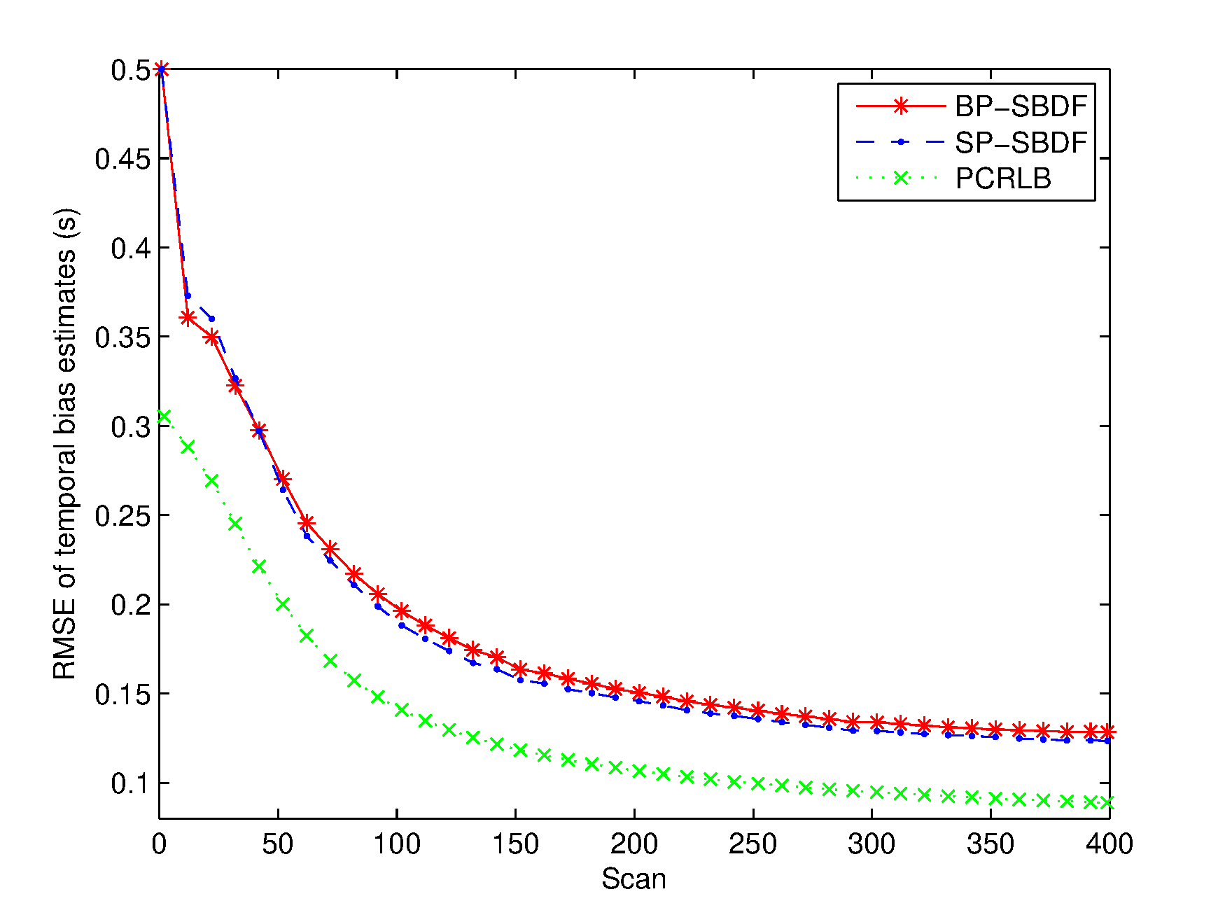
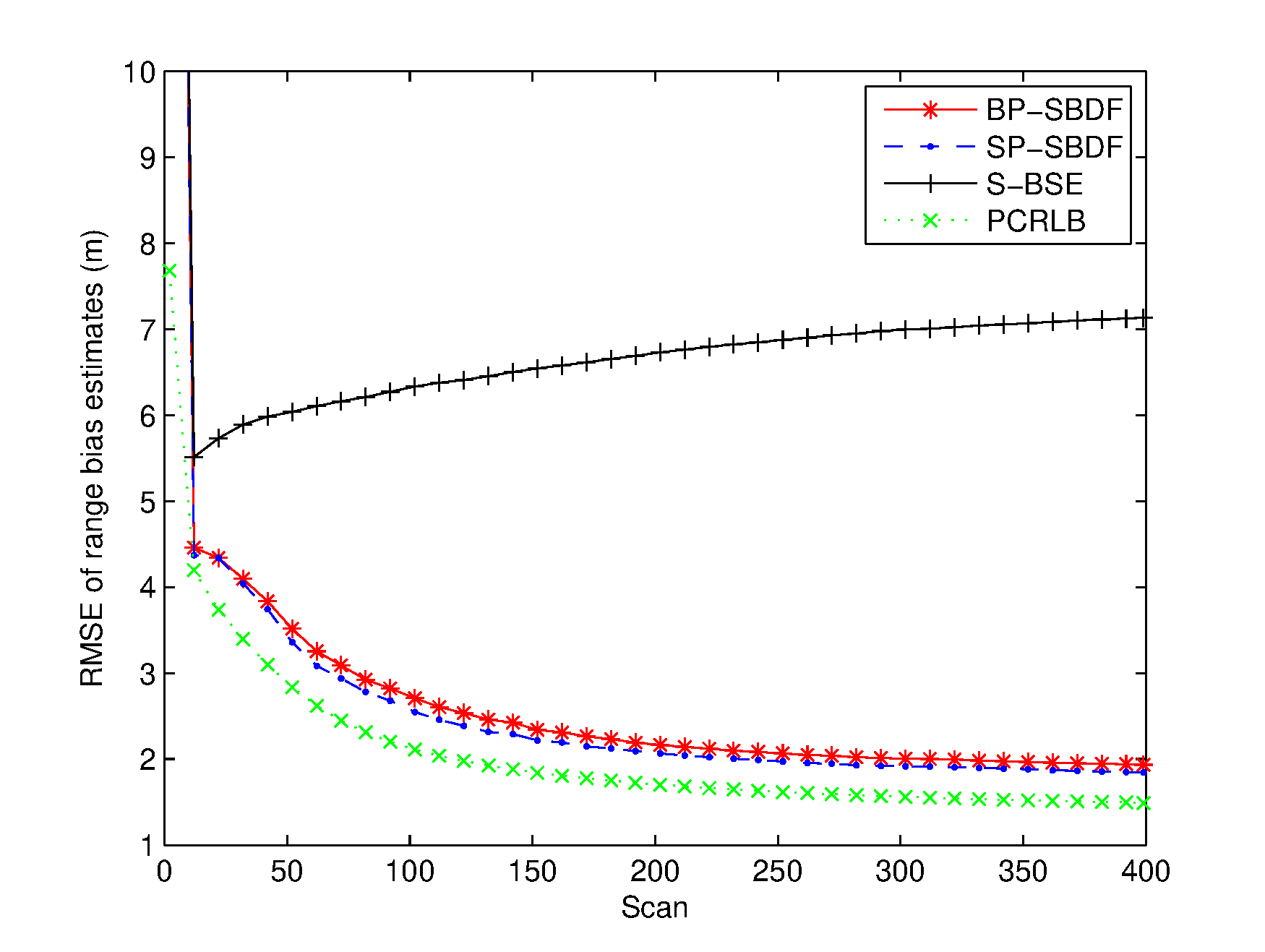
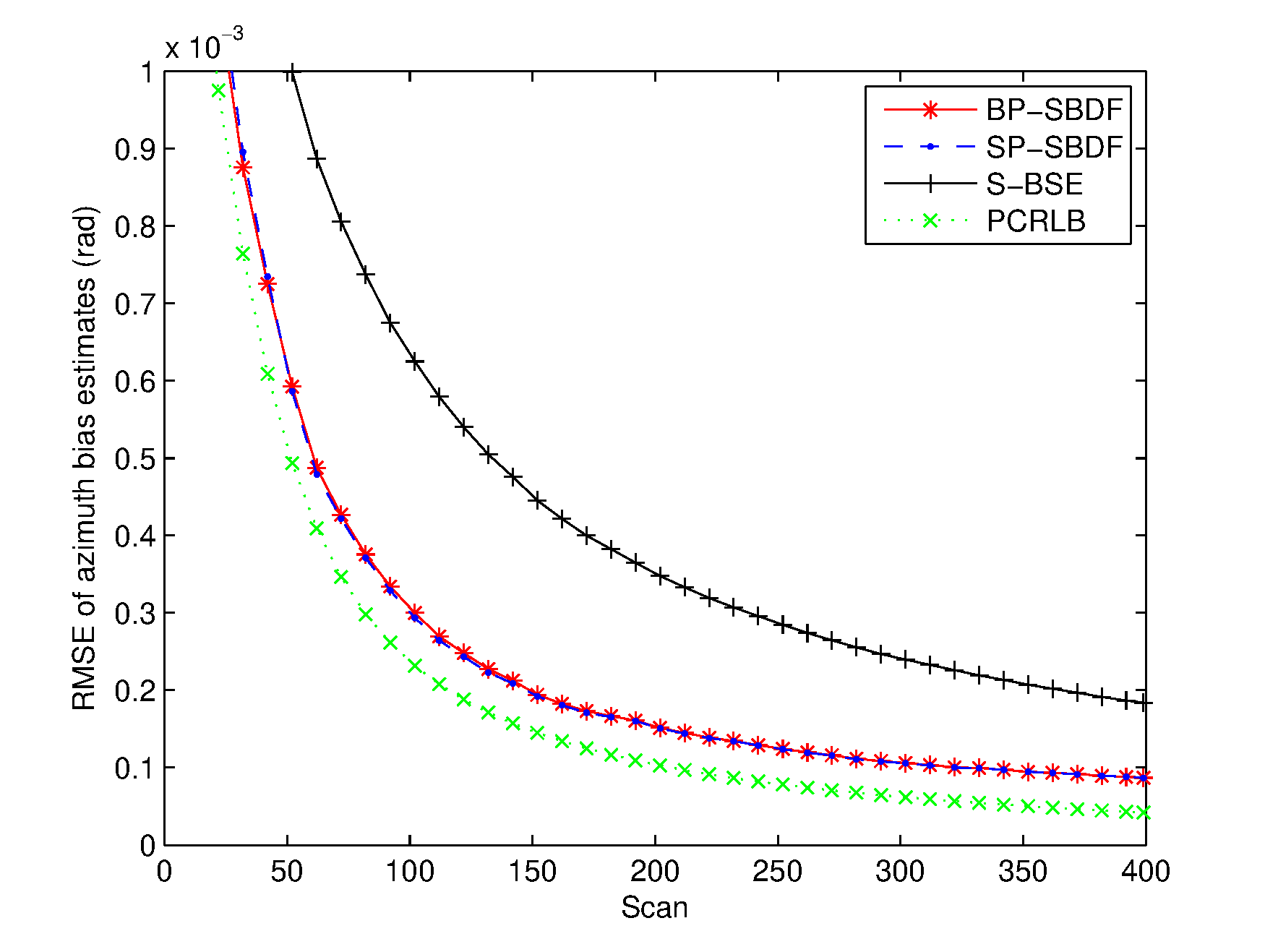
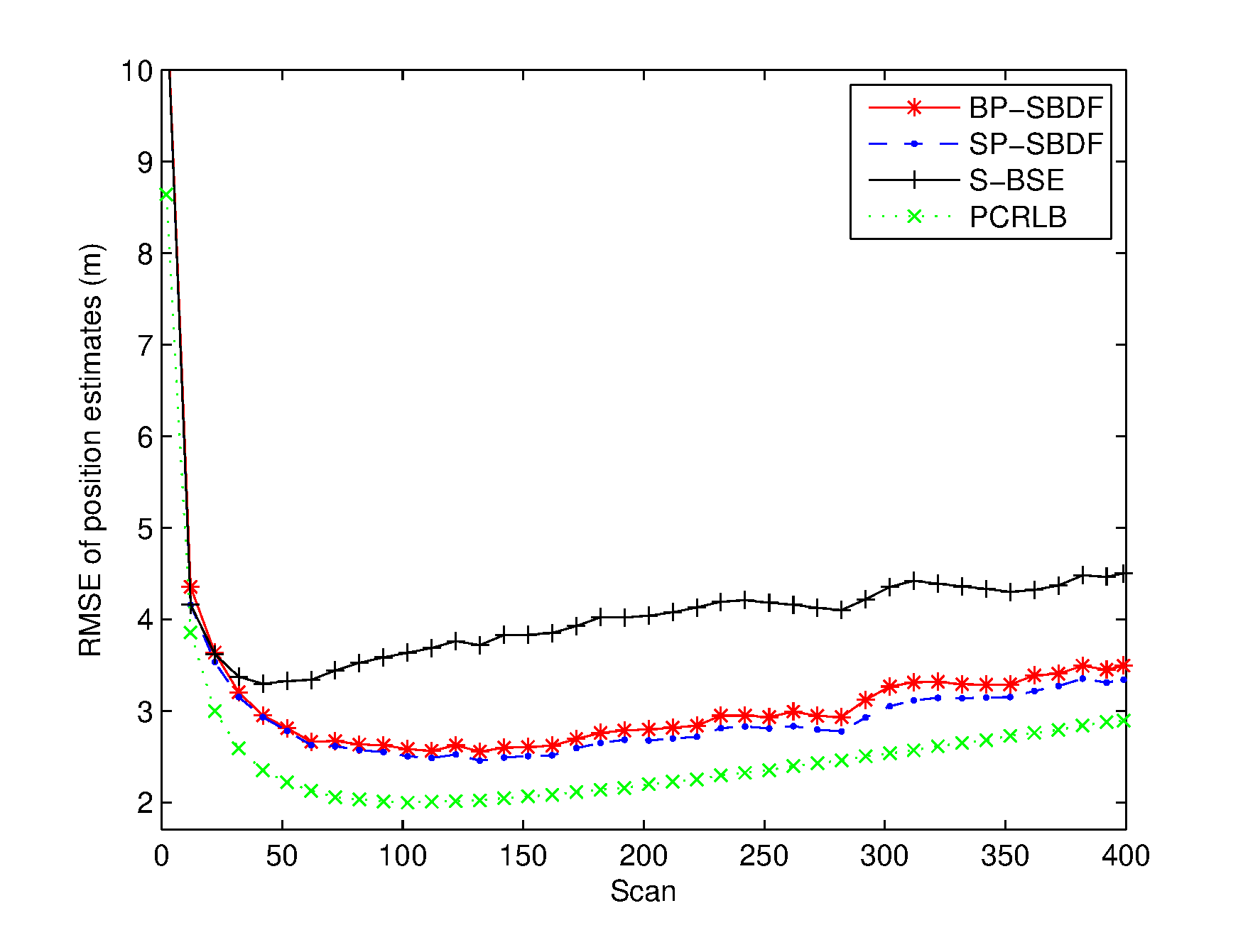
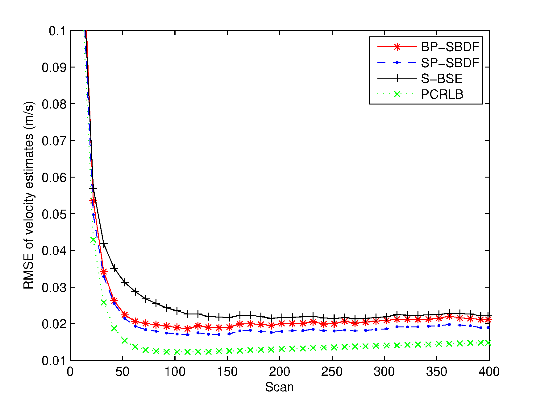
5.2 The Scenario with Relatively Small Temporal Bias

The RMSEs of the spatiotemporal bias and target state estimates are plotted in Figures 2 $-$ 6. The PCRLB is provided to quantify the theoretically achievable performance in this scenario. Additionally, time-averaged RMSEs of the proposed methods are listed in Table 1 for comparison. For fairness of comparison, two average running times are provided to compare the complexity of the proposed methods. One is the average running time required to handle the overall measurements of the two sensors, and the other is the average running time required to perform a single filtering process, which are also listed in Table 1.

Table 1 Performance comparison in scenario with relatively small temporal bias.

	RMSEs					Running Time
	Temporal Bias	Range Bias	Azimuth Bias	Position	Velocity	Overall	Single
	(s)	(m)	( $\times{10^{-4}}\;{\text{rad}}$ )	(m)	( ${{\text{m}}\mathord{\left/{\vphantom{{\text{m}}{\text{s}}}}\right.\kern-1.2pt}% {\text{s}}}$ )	(s)	( $\times{10^{-4}}{\rm{s}}$ )
BP-SBDF	0.1557	2.2431	1.7348	2.9410	0.0203	0.2177	5.4425
SP-SBDF	0.1502	2.1339	1.7163	2.8155	0.0183	0.4981	3.4000
S-BSE	$-$	6.7461	3.7369	4.0488	0.0226	$-$	$-$
PCRLB	0.1108	1.7534	1.2166	2.3393	0.0134	$-$	$-$

Figure 8 RMSE of temporal bias estimates of the BP-SBDF and SP-SBDF methods in Scenario II.

Figure 9 RMSE of range bias estimates of the BP-SBDF, SP-SBDF and S-BSE methods in Scenario II.

Figure 10 RMSE of azimuth bias estimates of the BP-SBDF, SP-SBDF and S-BSE methods in Scenario II.

Figure 11 RMSE of position estimates of the BP-SBDF, SP-SBDF and S-BSE methods in Scenario II.

Figure 12 RMSE of velocity estimates of the BP-SBDF, SP-SBDF and S-BSE methods in Scenario II.

Figure 13 Consistency test of the proposed methods in Scenario II.

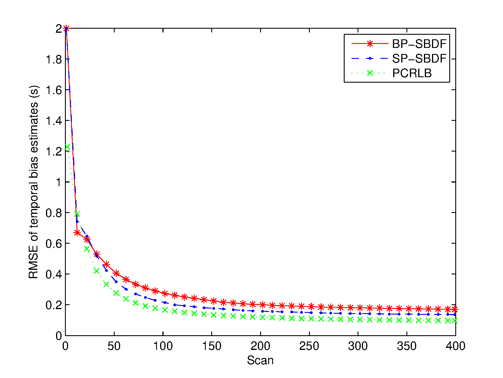
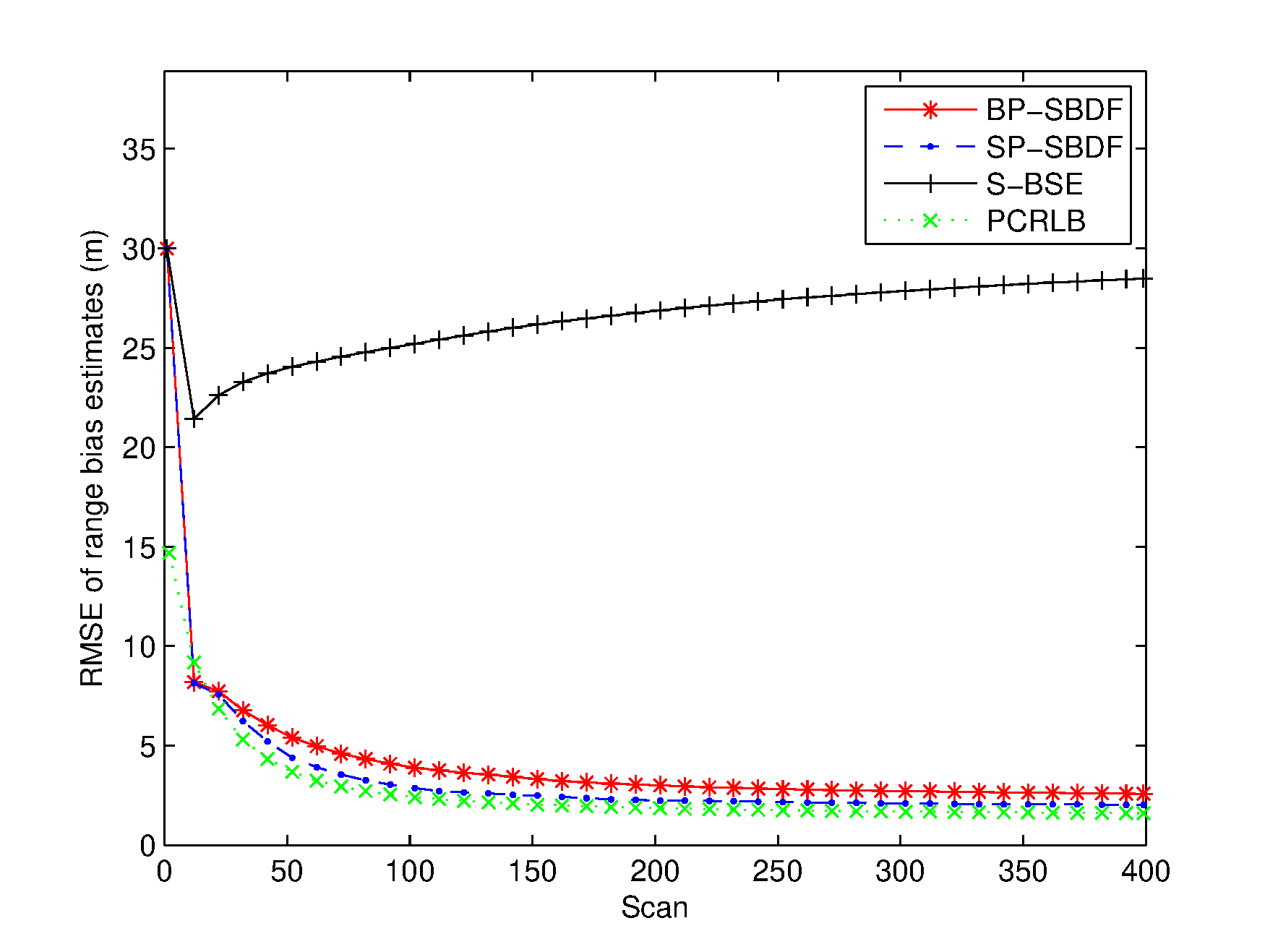
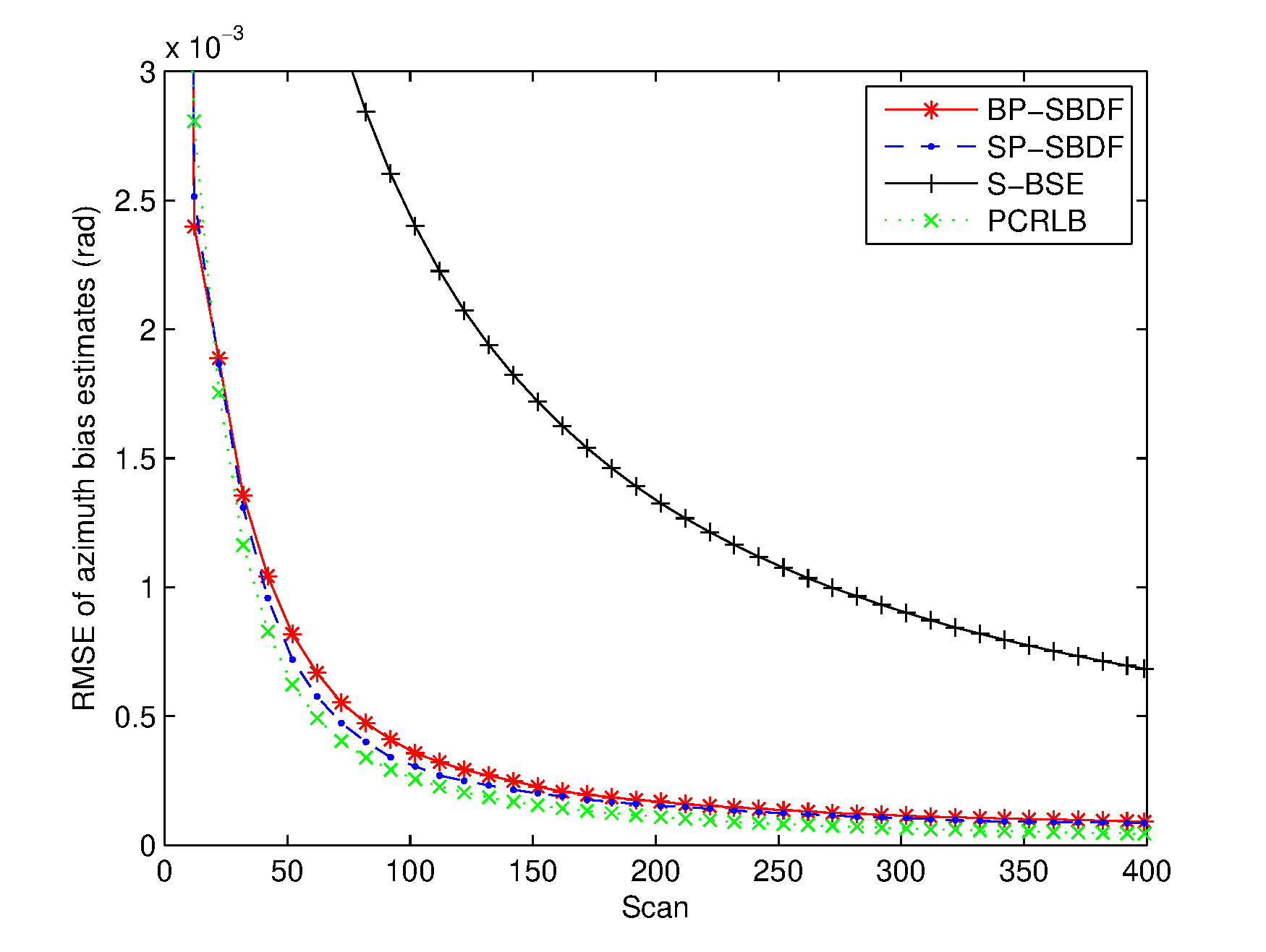
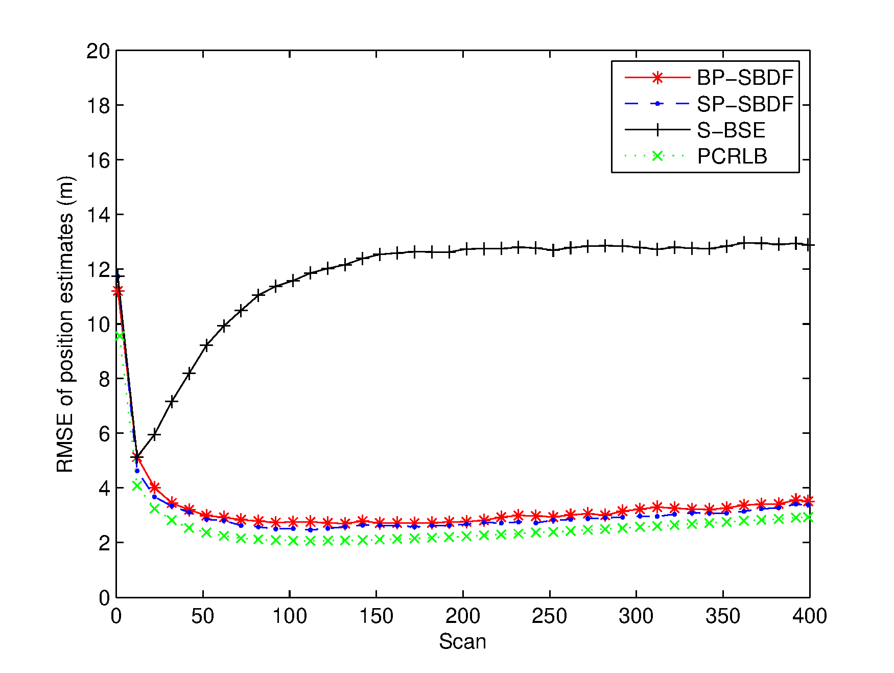
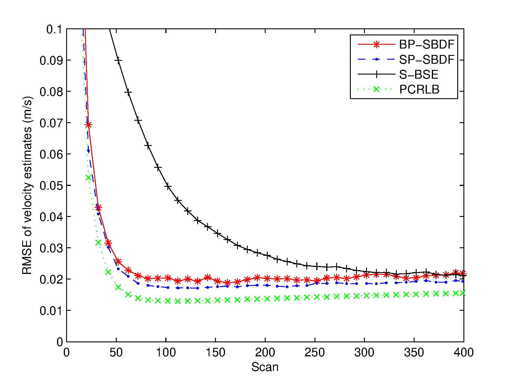
From Figures 3 $-$ 6, it can be seen that the spatial bias and target state RMSEs of the S-BSE method are larger than those of the BP-SBDF and SP-SBDF methods. As shown in Table 1, the improvements in time-averaged RMSEs of the range bias, azimuth bias, position and velocity of the BP-SBDF method are about $4.5030{\text{m}}$ , ${\text{2}}{\text{.0021}}\times{\text{1}}{{\text{0}}^{{\text{ - }}4}}\;{\text{% rad}}$ , $1.1078{\text{m}}$ and $0.0023\;{{\text{m}}\mathord{\left/{\vphantom{{\text{m}}{\text{s}}}}\right.% \kern-1.2pt}{\text{s}}}$ , respectively, with respect to those of the S-BSE method. Accordingly, the improvements in time-averaged RMSEs of the SP-SBDF method are about $4.6122{\text{m}}$ , ${\text{2}}{\text{.0206}}\times{\text{1}}{{\text{0}}^{{\text{ - }}4}}\;{\text{% rad}}$ , $1.2333{\text{m}}$ and $0.0043\;{{\text{m}}\mathord{\left/{\vphantom{{\text{m}}{\text{s}}}}\right.% \kern-1.2pt}{\text{s}}}$ , respectively. The S-BSE method does not consider and compensate for the temporal bias between sensors, which leads to estimation errors higher than those of the proposed methods. As a contrast, the proposed BP-SBDF and SP-SBDF methods properly compensate for the temporal bias while providing accurate spatiotemporal bias and target state estimates, both of which can reach the steady state rapidly, as shown in Figures 2 $-$ 6 and Table 1. Note that there still exists deviations between the RMSEs and the theoretical lower bounds. The main reason may lie in the high nonlinearity in the measurement equation.

Additionally, we can see that the SP-SBDF method performs slightly better than the BP-SBDF method. The BP-SBDF method estimates the state once using all the measurements collected in a fusion period based on the prior state updated in the previous fusion period. While the SP-SBDF method updates the state once a measurement is received, where the state updated by the previous measurement is used as prior information, which is more accurate than the state estimate of the previous fusion period. This results in the slight superiority of the SP-SBDF method over the BP-SBDF method in estimation accuracy.

As shown in Table 1, the SP-SBDF method requires more time to handle all measurements from the two sensors than the BP-SBDF method. This can be explained by the different measurement processing schemes of the two methods. The BP-SBDF method only utilizes the UKF at the measurement times of sensor 1 to generate the augmented state estimates, so only 400 calls of the UKF are required. On the contrary, the SP-SBDF method calls the UKF 1465 times to generate the augmented state estimates when handling the same number of measurements, which results in the SP-SBDF method requiring more running time than the BP-SBDF method. If we focus on a single filtering process, we can see that the running time required by the SP-SBDF method is less than that of the BP-SBDF method. This is because that the measurement dimension in the BP-SBDF method is higher than that in the SP-SBDF method.

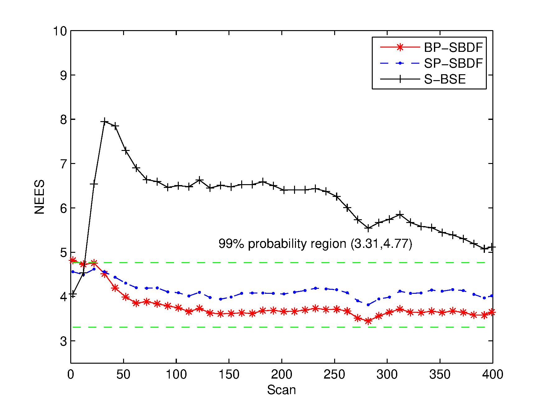
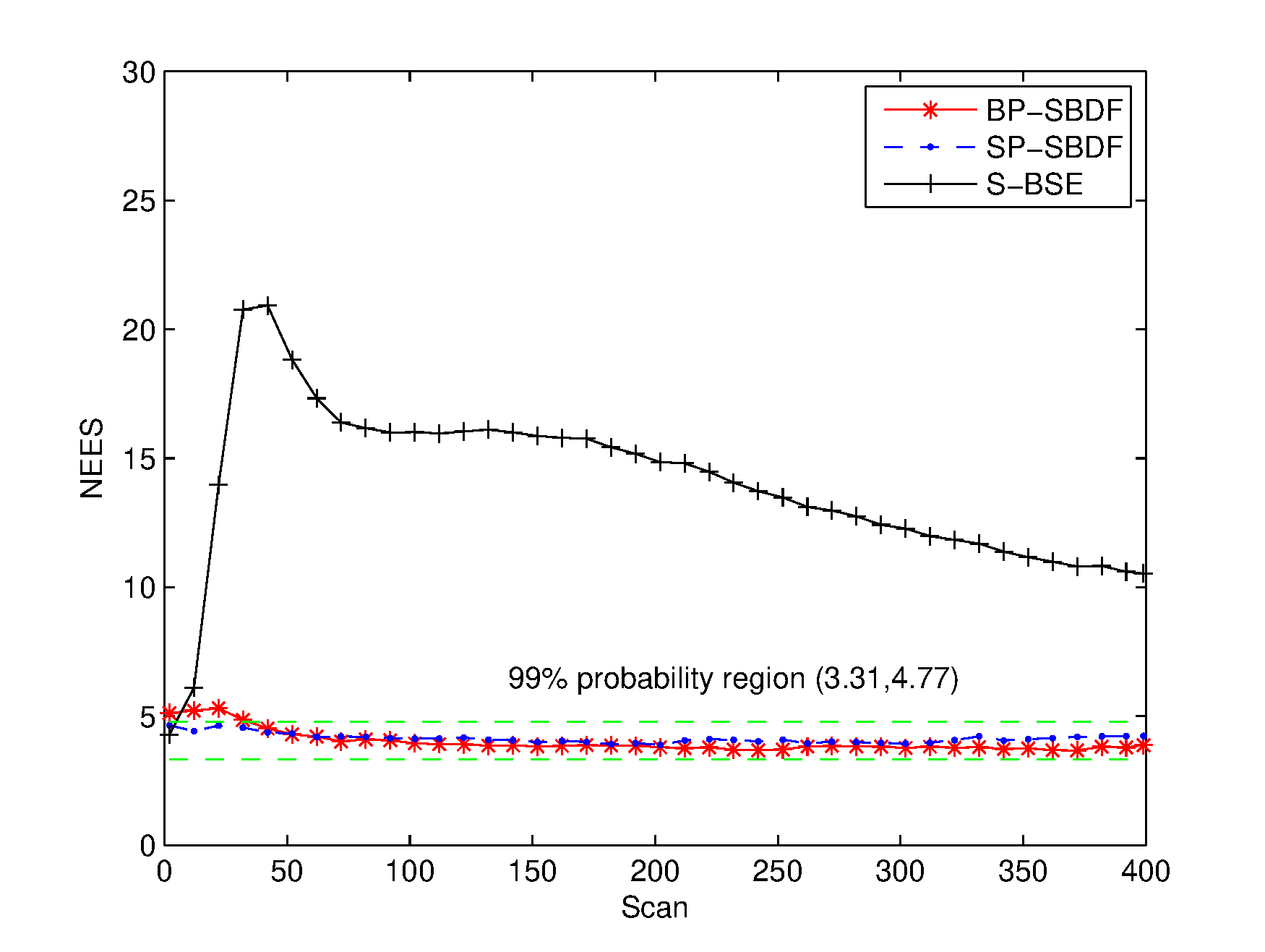
The consistency of the methods is examined based on the evaluation of the NEES, as shown in Figure 7.

Here, we use the two-sided $99\%$ probability region. The results in Figure 7 show the inconsistency of the S-BSE method since its NEES values are mostly outside the region of 99% . The proposed methods are consistent since their NEES values fall within the probability region. Therefore, the proposed methods can fuse the multisensor measurements to provide accurate and consistent state estimation while compensating for the spatiotemporal biases.

5.3 The Scenario with Relatively Large Temporal Bias

This scenario aims to evaluate the effects on the estimation performance when the temporal bias increases. Additionally, the measurements may be reported in the wrong order according to the time stamps since the time delays of sensors differ a lot. This scenario is also used to evaluate whether the proposed methods can still perform well when the measurements are in wrong order. The RMSEs of the spatiotemporal bias and state estimates and the NEES of the tracking filters are shown in Figures 8 $-$ 13, respectively. Time-averaged RMSEs and the average running times of the proposed methods are listed in Table 2 for comparison.

Table 2 Performance comparison in scenario with relatively large temporal bias.

	RMSEs					Running Time
	Temporal Bias	Range Bias	Azimuth Bias	Position	Velocity	Overall	Single
	(s)	(m)	( $\times{10^{-4}}\;{\text{rad}}$ )	(m)	( ${{\text{m}}\mathord{\left/{\vphantom{{\text{m}}{\text{s}}}}\right.\kern-1.2pt}% {\text{s}}}$ )	(s)	( $\times{10^{-4}}{\rm{s}}$ )
BP-SBDF	0.2223	3.1206	2.0088	2.9882	0.0204	0.2245	5.6125
SP-SBDF	0.1680	2.3662	1.7675	2.8165	0.0183	0.5054	3.4498
S-BSE	$-$	26.9249	14.2627	12.4416	0.0320	$-$	$-$
PCRLB	0.1258	1.9367	1.2223	2.3867	0.0141	$-$	$-$

From Figures 9 $-$ 13, it can be seen that the improper processing of the temporal bias degrades the performance of the S-BSE method, resulting in estimation error much higher than the PCRLB and NEES outside the $99\%$ probability region. Additionally, as can be seen in Figures 9 $-$ 10, the estimation errors of the range bias of the S-BSE method become larger with time, while those of the azimuth bias become smaller. This is because that the target in this scenario is moving away from the sensors. The impact of the temporal bias on the range bias estimation becomes large with the increase of the target range, while the impact on the azimuth bias is the opposite.

On the contrary, the proposed methods can provide accurate and consistent spatiotemporal bias and target state estimation simultaneously. As shown in Table 2, the improvements from the BP-SBDF and SP-SBDF methods over the S-BSE method are about $23.8043-24.5587{\text{m}}$ in range bias RMSE, $12.2539\times{10^{-4}}-12.4952\times{10^{-4}}\;{\text{rad}}$ in azimuth bias RMSE, $9.4534-9.6251{\text{m}}$ in position RMSE, and $0.0116-0.0137\;{{\text{m}}\mathord{\left/{\vphantom{{\text{m}}{\text{s}}}}% \right.\kern-1.2pt}{\text{s}}}$ in velocity RMSE, respectively. Since the temporal bias is properly compensated by the proposed methods, the spatiotemporal bias and target state estimation errors keep small values, which also shows that the proposed methods can perform well even when the measurements are reported in the wrong order. As a consequence, the above results confirm the necessity of our methods to consider the temporal bias between sensors to perform correct data fusion. Additionally, the SP-SBDF method still performs slightly better but requires a little more computation load than the BP-SBDF method when handling all measurements from the two sensors, which are $0.5054{\text{s}}$ and $0.2245{\text{s}}$ , respectively. Also, the running time required by the SP-SBDF method in a single filtering process is less than that of the BP-SBDF method, which are $3.4498\times{10^{-4}}{\rm{s}}$ and ${\rm{5}}{\rm{.6125}}\times{10^{-4}}{\rm{s}}$ , respectively. These simulation results agree with those in Section 5.2, which means the proposed methods can perform well irrespective of whether the temporal bias is small or large.

6. Conclusions

In this paper, two spatiotemporal bias compensation methods were proposed to compensate for the spatiotemporal biases and fuse the multisensor measurements to produce accurate target state estimates. The general case where sensors have different and varying sampling periods was considered. The augmented state vectors consist of target states and spatiotemporal biases of multisensor. The measurement equations for the batch processing and sequential processing schemes were formulated as functions of both target states and spatiotemporal biases according to their relationship, which enables simultaneous spatiotemporal bias estimation and data fusion. The UKF was employed to handle the nonlinearity of the measurements and estimate spatiotemporal biases and target states simultaneously. Simulation results demonstrated that the proposed methods can provide accurate spatiotemporal bias and target state estimation simultaneously. Due to high nonlinearities in the measurement equations, the performance of the proposed methods has not reached the PCRLB. Further improving the performance of the spatiotemporal bias estimation is a topic of future efforts.

Data Availability Statement

Data will be made available on request.

Funding

This work was supported by the National Natural Science Foundation of China under Grant 61671181.

Conflicts of Interest

The authors declare no conflicts of interest.

Ethical Approval and Consent to Participate

Not applicable.

References

Bar-Shalom, Y., Willett, P. K., & Tian, X. (2011). Tracking and data fusion (Vol. 11). Storrs, CT, USA:: YBS publishing.
[Google Scholar]
Bar-Shalom, Y., Li, X. R., & Kirubarajan, T. (2004). Estimation with applications to tracking and navigation: theory algorithms and software. John Wiley & Sons.
[Google Scholar]
Ge, Q., Shao, T., Yang, Q., Shen, X., & Wen, C. (2016). Multisensor nonlinear fusion methods based on adaptive ensemble fifth-degree iterated cubature information filter for biomechatronics. IEEE Transactions on Systems, Man, and Cybernetics: Systems, 46(7), 912-925.
[CrossRef] [Google Scholar]
Khaleghi, B., Khamis, A., Karray, F. O., & Razavi, S. N. (2013). Multisensor data fusion: A review of the state-of-the-art. Information Fusion, 14(1), 28-44.
[CrossRef] [Google Scholar]
Chen, B., Hu, G., Ho, D. W., Zhang, W. A., & Yu, L. (2016). Distributed robust fusion estimation with application to state monitoring systems. IEEE Transactions on Systems, Man, and Cybernetics: Systems, 47(11), 2994-3005.
[CrossRef] [Google Scholar]
Yu, D., Xia, Y., Li, L., Xing, Z., & Zhu, C. (2019). Distributed covariance intersection fusion estimation with delayed measurements and unknown inputs. IEEE Transactions on Systems, Man, and Cybernetics: Systems, 51(8), 5165-5173.
[CrossRef] [Google Scholar]
Lin, X., Pan, X., Sun, W., Liu, L., & Chen, X. (2022). Multi-scale asynchronous fusion algorithm for multi-sensor integrated navigation system. Proceedings of the Institution of Mechanical Engineers, Part I: Journal of Systems and Control Engineering, 236(9), 1709-1723.
[CrossRef] [Google Scholar]
Lin, H., & Sun, S. (2017). Distributed fusion estimator for multisensor multirate systems with correlated noises. IEEE Transactions on Systems, Man, and Cybernetics: Systems, 48(7), 1131-1139.
[CrossRef] [Google Scholar]
Burke, J. (1966). The SAGE real quality control fraction and its interface with BUIC II/BUIC III. MITRE Corporation, Technical report 308.
[Google Scholar]
Leung, H., Blanchette, M. & Harrison, C. (1994). A least squares fusion of multiple radar data. In Proceedings of Radar 94, Paris, France, (pp. 498–508.)
[Google Scholar]
Zhou, Y., Leung, H., & Blanchette, M. (1999). Sensor alignment with earth-centered earth-fixed (ECEF) coordinate system. IEEE Transactions on Aerospace and Electronic systems, 35(2), 410-418.
[CrossRef] [Google Scholar]
Zheng, Z. W., & Zhu, Y. S. (2004). New least squares registration algorithm for data fusion. IEEE Transactions on Aerospace and Electronic Systems, 40(4), 1410-1416.
[CrossRef] [Google Scholar]
Zhou, Y., Leung, H., & Yip, P. C. (1997). An exact maximum likelihood registration algorithm for data fusion. IEEE Transactions on Signal Processing, 45(6), 1560-1573.
[CrossRef] [Google Scholar]
Okello, N., & Ristic, B. (2003). Maximum likelihood registration for multiple dissimilar sensors. IEEE Transactions on Aerospace and Electronic Systems, 39(3), 1074-1083.
[CrossRef] [Google Scholar]
Rafati, A., Moshiri, B., & Rezaei, J. (2007, July). A new algorithm for general asynchronous sensor bias estimation in multisensor-multitarget systems. In 2007 10th International Conference on Information Fusion (pp. 1-8). IEEE.
[CrossRef] [Google Scholar]
Helmick, R. E., & Rice, T. R. (1993). Removal of alignment errors in an integrated system of two 3-D sensors. IEEE Transactions on Aerospace and Electronic systems, 29(4), 1333-1343.
[CrossRef] [Google Scholar]
Nabaa, N., & Bishop, R. H. (1999). Solution to a multisensor tracking problem with sensor registration errors. IEEE Transactions on Aerospace and Electronic systems, 35(1), 354-363.
[CrossRef] [Google Scholar]
Song, Q. He, Y. & Yang, J. (2007). An augmented state target tracking algorithm with systematic errors based on the unscented Kalman filter. Journal of Projectiles, Rockets, Missiles and Guidance, no. 3, (pp. 311–316).
[Google Scholar]
Liu, J., Zuo, Y., & Xue, A. (2013, July). An ASEKF algorithm for 2D and 3D radar registration. In Proceedings of the 32nd Chinese Control Conference (pp. 4758-4761). IEEE.https://ieeexplore.ieee.org/abstract/document/6640261
[Google Scholar]
Furgale, P., Rehder, J., & Siegwart, R. (2013, November). Unified temporal and spatial calibration for multi-sensor systems. In 2013 IEEE/RSJ International Conference on Intelligent Robots and Systems (pp. 1280-1286). IEEE.
[CrossRef] [Google Scholar]
Rehder, J., Beardsley, P., Siegwart, R., & Furgale, P. (2014, September). Spatio-temporal laser to visual/inertial calibration with applications to hand-held, large scale scanning. In 2014 IEEE/RSJ International Conference on Intelligent Robots and Systems (pp. 459-465). IEEE.
[CrossRef] [Google Scholar]
Rehder, J., Siegwart, R., & Furgale, P. (2016). A general approach to spatiotemporal calibration in multisensor systems. IEEE Transactions on Robotics, 32(2), 383-398.
[CrossRef] [Google Scholar]
Nocedal, J., & Wright, S. J. (Eds.). (1999). Numerical optimization. New York, NY: Springer New York.
[Google Scholar]
You, H., Hongwei, Z., & Xiaoming, T. (2013). Joint systematic error estimation algorithm for radar and automatic dependent surveillance broadcasting. IET Radar, Sonar & Navigation, 7(4), 361-370.
[CrossRef] [Google Scholar]
Li, S., Cheng, Y., Brown, D., Tharmarasa, R., Zhou, G., & Kirubarajan, T. (2019). Comprehensive time-offset estimation for multisensor target tracking. IEEE Transactions on Aerospace and Electronic Systems, 56(3), 2351-2373.
[CrossRef] [Google Scholar]
Li, M., & Mourikis, A. I. (2013, May). 3-D motion estimation and online temporal calibration for camera-IMU systems. In 2013 IEEE International Conference on Robotics and Automation (pp. 5709-5716). IEEE.
[CrossRef] [Google Scholar]
Li, W., & Leung, H. (2004). Simultaneous registration and fusion of multiple dissimilar sensors for cooperative driving. IEEE Transactions on Intelligent Transportation Systems, 5(2), 84-98.
[CrossRef] [Google Scholar]
Li, W., Leung, H., & Zhou, Y. (2004). Space-time registration of radar and ESM using unscented Kalman filter. IEEE Transactions on Aerospace and Electronic Systems, 40(3), 824-836.
[CrossRef] [Google Scholar]
Huang, D., & Leung, H. (2005). An expectation-maximization-based interacting multiple model approach for cooperative driving systems. IEEE Transactions on Intelligent Transportation Systems, 6(2), 206-228.
[CrossRef] [Google Scholar]
Bu, S., & Zhou, G.(2016). Spatiotemporal registration for multi-sensor fusion systems. In Proceedings of the International Conference on Artificial Intelligence and Computer Science, Guilin, China (pp. 333–339).
[Google Scholar]
Bu, S., Zhou, C., & Zhou, G. (2019). Simultaneous spatiotemporal bias and state estimation for asynchronous multi‐sensor system. The Journal of Engineering, 2019(19), 5824-5828.
[CrossRef] [Google Scholar]
Tichavsky, P., Muravchik, C. H., & Nehorai, A. (1998). Posterior Cramér-Rao bounds for discrete-time nonlinear filtering. IEEE Transactions on Signal Processing, 46(5), 1386-1396.
[CrossRef] [Google Scholar]
Gongjian, Z. H. O. U., Changjun, Y. U., Naigang, C. U. I., & Taifan, Q. U. A. N. (2012). A tracking filter in spherical coordinates enhanced by de-noising of converted Doppler measurements. Chinese Journal of Aeronautics, 25(5), 757-765.
[CrossRef] [Google Scholar]
Blair, W. D. (2008, June). Design of nearly constant velocity track filters for tracking maneuvering targets. In 2008 11th International Conference on Information Fusion (pp. 1-7). IEEE.
[Google Scholar]
You, H., Jianjuan, X., & Xin, G. (2016). Radar data processing with applications. John Wiley & Sons.
[Google Scholar]
Angrisani, L., D'Apuzzo, M., & Moriello, R. S. L. (2005, May). The unscented transform: a powerful tool for measurement uncertainty evaluation. In Proceedings of the 2005 IEEE International Workshop on Advanced Methods for Uncertainty Estimation in Measurement, 2005. (pp. 27-32). IEEE.
[CrossRef] [Google Scholar]
Challa, S. (2011). Fundamentals of object tracking. Cambridge University Press.
[Google Scholar]
Lerro, D., & Bar-Shalom, Y. (1993). Tracking with debiased consistent converted measurements versus EKF. IEEE Transactions on Aerospace and Electronic systems, 29(3), 1015-1022.
[CrossRef] [Google Scholar]
Longbin, M., Xiaoquan, S., Yiyu, Z., Kang, S. Z., & Bar-Shalom, Y. (1998). Unbiased converted measurements for tracking. IEEE Transactions on Aerospace and Electronic Systems, 34(3), 1023-1027.
[CrossRef] [Google Scholar]
Duan, Z., Han, C., & Li, X. R. (2004). Comments on" unbiased converted measurements for tracking". IEEE Transactions on Aerospace and Electronic systems, 40(4), 1374.
[CrossRef] [Google Scholar]
Van Trees, H. L. (2004). Detection, estimation, and modulation theory, part I: detection, estimation, and linear modulation theory. John Wiley & Sons.
[Google Scholar]

Cite This Article

APA Style

Zhou, G., Bu, S., & Kirubarajan, T. (2024). Simultaneous Spatiotemporal Bias Compensation and Data Fusion for Asynchronous Multisensor Systems. Chinese Journal of Information Fusion, 1(1), 16–32. https://doi.org/10.62762/CJIF.2024.361881

Article Metrics

Citations:

Google Scholar

Crossref

Scopus

Web of Science

Article Access Statistics:

PDF Downloads: 708

Publisher's Note

ICCK stays neutral with regard to jurisdictional claims in published maps and institutional affiliations.

Rights and permissions

Copyright © 2024 by the Author(s). Published by Institute of Central Computation and Knowledge. This article is an open access article distributed under the terms and conditions of the Creative Commons Attribution (CC BY) license (https://creativecommons.org/licenses/by/4.0/), which permits use, sharing, adaptation, distribution and reproduction in any medium or format, as long as you give appropriate credit to the original author(s) and the source, provide a link to the Creative Commons licence, and indicate if changes were made.

Chinese Journal of Information Fusion

ISSN: 2998-3371 (Online) | ISSN: 2998-3363 (Print)

Email: [email protected]

Portico

All published articles are preserved here permanently:
https://www.portico.org/publishers/icck/

Table of Content

1. Introduction

2. Problem Formulation

3. Simultaneous Spatiotemporal Bias Compensation and Data Fusion

3.1 Augmented State Equation

3.2 The Measurement Equation

3.2.1 Measurement Equation for Batch Processing Scheme

3.2.2 Measurement Equation for Sequential Processing Scheme

3.3 Filtering Process

3.4 Filter Initialization

4. Lower Bound of Performance

5. Simulation Results

5.1 Simulation Parameters

5.2 The Scenario with Relatively Small Temporal Bias

5.3 The Scenario with Relatively Large Temporal Bias

6. Conclusions

Google Scholar

Crossref

Scopus

Web of Science

We use cookies