


Chinese Journal of Information Fusion
ISSN: 2998-3371 (Online) | ISSN: 2998-3363 (Print)
Email: [email protected]

The ocean is the cradle of life, the natural cornucopia and the main avenue for transportation. It provides water circulation for life, stores energy for the earth and offers sufficient space for human beings to explore nature and promote economic transformation. Developing, utilizing, and managing the ocean have become effective means for countries to address issues such as population growth, environmental pollution, and resource shortages. Illegal, unreported and unregulated fishing is one of the most serious threats to the sustainable development of marine resources and is capable of causing immeasurable damage to marine biodiversity and ecosystems. Marine domain awareness requires the use of data and information from marine intelligence sources to continuously monitor and track fisheries, uncover relevant illegal activities in a timely manner and effectively curb and combat them.
In recent years, the wide application of automatic identification systems (AISs) [1] on ships has gradually led to a new era in maritime traffic monitoring. An AIS not only functions as a global tracking system but also incorporates navigation equipment that utilizes modern technology for automated ship-to-shore and ship-to-ship identification. Through the tracking system, the ship broadcasts its own dynamic (such as longitude, latitude, ground speed, ground heading, navigation status, etc.) and static information (such as MMSI number, ship size, ship type, etc.), reducing the risk of collision between maritime ships through the exchange of ship status information to monitor their navigational intentions while helping maritime personnel monitor ship mobility. Although AISs were originally designed for security purposes, it soon became obvious that if relevant technical means could be developed to effectively extract, detect and analyze relevant information from these data streams to help the maritime department monitor ships at sea, the potential of these vast amounts of data would be intriguing. However, manually processing such vast amounts of data is impractical. Therefore, despite the inherent challenges, AIS data must be analyzed using artificial intelligence-based methods.
Trajectory classification is a research domain focused on analyzing tracking data of moving objects to develop classifiers that can distinguish various motion patterns. In recent years, the rapid development of big spatiotemporal ocean data has gradually shifted the focus of corresponding researchers to the ocean field. However, due to the limitations of ship AIS data acquisition, there are few studies on trajectory classification of ship AIS data. Generally, the research methods involved at present are mainly divided into two groups: traditional machine learning-based methods and deep learning-based methods.
In some studies, researchers have mainly used traditional machine learning as the basis for methods for ship trajectory classification and improved the experimental results by implementing innovative and beneficial modifications to these traditional methods. Liu et al. [2] proposed a ship trajectory classification algorithm based on the K-nearest neighbor (KNN) algorithm. The trajectories of the KNN classification samples are obtained through the preliminary clustering of ship trajectories, which are then classified by taking the comprehensive distance as the distance between trajectories in the KNN classification. The experimental results show that this method is highly suitable for inland river ship trajectory classification. Guan et al. [3] proposed using the Light Gradient Boosting Machine (LightGBM) to establish a fishing vessel type recognition model and extracted more than 60 features from the AIS data, including speed, heading, and position and speed change. The accuracy of the model on the AIS dataset from the north of the South China Sea in 2018 was 95.68%, which was higher than that of other advanced algorithms such as XGBoost; Krüger et al. [4] calculated various ship characteristics through latitude, longitude, speed and other attributes based on five relevant AIS datasets, and evaluated the experimental results by using five classifiers, including decision tree, fuzzy rules, K-nearest neighbor, neural network and naive Bayes, three groups of classification labels and the accuracy of two evaluation criteria. The experimental results showed that the decision tree, fuzzy rules and K-nearest neighbor classification methods had high accuracy, and the classification results were deeply analyzed and summarized.
The final accuracy of traditional machine learning methods largely depends on the quality of feature engineering performed before the classifier, but the features obtained with feature engineering need to be extracted manually. Thus, these methods not only require human experts to design and combine the features but also require researchers to spend considerable time and energy extracting them. In addition, different application scenarios require the extraction of different effective features to express the corresponding data. Consequently, traditional machine learning methods are generally more suitable for specific application scenarios and tasks involving relatively small datasets.
In recent years, the popularization of deep learning technology has led to the wide use of convolutional neural networks (CNNs) and recurrent neural networks (RNNs) in various research fields. The former has achieved great success in the field of computer vision [5] for classifying and recognizing image data, while the latter has played a more significant role in the field of time series in the classification and prediction of sequence data [6]. Arasteh et al. [7] proposed a CNN model named FishNET for ship trajectory classification. The model uses a set of invariant spatiotemporal feature sequences extracted from ship AIS trajectory data for training and was applied to a large, 4-year real fishing vessel dataset collected in the United States and Denmark to identify the gill net, purse seine, trawl and longline fishing behaviors of fishing vessels. Kontopoulos et al. [8] proposed a new high-precision AIS message flow trajectory classification method. By conceptualizing the ship activity classification problem as an image classification task and using the VGG16, InceptionV3, NASNetLarge and DenseNet201 models to address it, the authors conducted experiments and found that the VGG16 model achieved the highest classification accuracy and that the InceptionV3 model achieved the lowest processing delay. Shen et al. [9] proposed a method to classify the trajectory activity of the three primary types of fishing vessels along the coast of Taiwan by using a multilayer bidirectional LSTM model. Through experiments, the authors found that the selection of key features from AIS data can effectively improve the classification accuracy and suggested including an RNN model to learn better spatial representation.
Different from the traditional machine learning methods, deep learning methods can transform the original data into more abstract, more complex and higher-level expressions through nonlinear models and can learn more complex functions through sufficient model combinations. Therefore, they can replace manual feature extraction methods and automatically learn the features that best reflect differences from a large amount of data in an end-to-end manner. In addition, deep learning methods are suitable for learning tasks with a large amount of data and have good generalizability with new data sources and new learning tasks. Therefore, based on these characteristics, deep learning methods are ideal for trajectory classification using ship AIS data.
The development of artificial intelligence technology and the proposal of a series of deep learning methods have provided more possibilities for ship behavior analysis using big data-based trajectory features. At present, ship motion trajectory classification methods based on deep learning are mainly divided into two domains: the computer-vision domain and the time-series domain. Methods based on the former determine the trajectory category of the image by transforming the time-series trajectory information into a static trajectory image. This method places greater emphasis on the geometric information of ship motion trajectory; however, the ability to capture ship motion feature information is poor and the recognition accuracy largely depends on the distribution of the data and is low for atypical motion trajectories. Time-series domain-based methods, meanwhile, directly take the time-series trajectory information as the input to determine the trajectory category. These methods place greater emphasis on changes in the motion state of the ship, but the classification effect is poor in cases where the motion characteristics of different types of trajectories are similar.
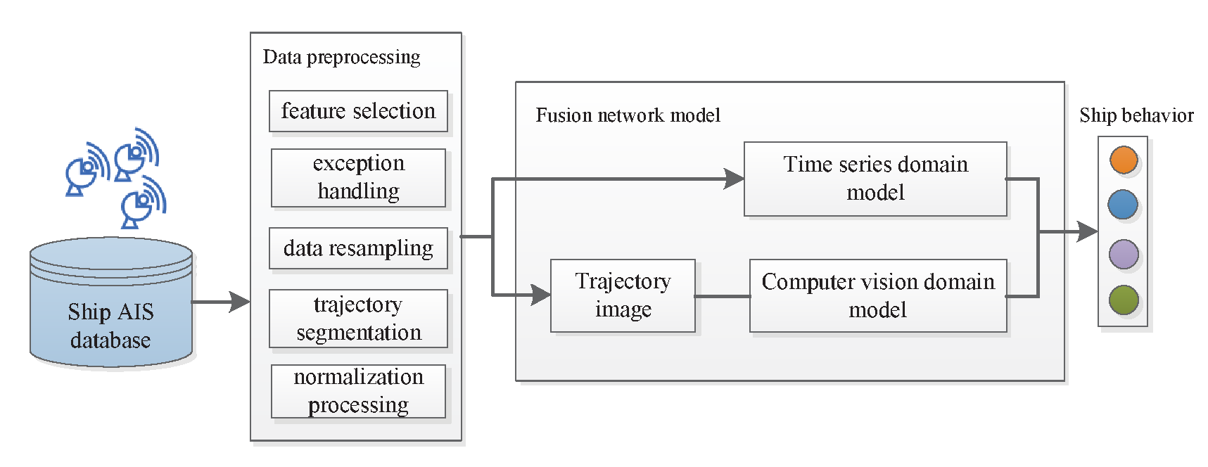
To realize the accurate classification and recognition of ship behavior patterns, this paper considers the motion state information and the trajectory shape information generated during ship motion, designs a fusion model framework combining the computer-vision and time-series domains, and proposes the corresponding optimizations and improvements. The overall framework of this method is shown in Figure 1.
Considering the limited field types of ship status in the data set source and that some ship statuses do not have specific characteristics in the behavior patterns or have no actual research value, such as the ship grounding and losing control, this paper mainly realizes the identification of four different ship behavior patterns from AIS data [10]:
1) Anchoring: Anchoring is a key operation in ship navigation, defined as the safe berthing method in which the combined grasping force of the anchor and anchor chain is greater than the sum of external forces, preventing the ship from moving as a result. Anchoring is often related to the berthing, tide, loading and unloading, quarantining and sheltering of ships. During such activities, the ship is anchored in an offshore anchorage area.The ship tends to move around the anchor and presents a circular or semicircular track shape in different directions, as shown in Figure 2(a), in which the anchor is approximately located in the middle of the circle. The circular motion of the ship around the anchor may be caused by the influence of wind, the tide or ocean currents. Depending on the ship type, the ground speed is approximately 0.0-3.0 knots.
2) Mooring: Mooring refers to the process of using equipment to make the ship stop at the berth. Mooring is related to permanent structures of fixed vessels, such as wharves, anchor buoys and mooring buoys. In such activities, the ship is constrained not only by its anchor but also, for example, by the mooring buoy. Therefore, compared with the anchoring pattern, the movement of the ship is more limited during mooring, and the ship position is "close" to the mooring equipment, as shown in Figure 2(b). This slight movement arises due to the influence of wind and ocean currents, and the ground speed generally does not exceed 1.0 or 2.0 knots.
3) Sailing: A ship is considered to be in sailing when it is not grounded, anchored or tied to the wharf, shore or other stationary objects. In such activities, the trajectory of the ship usually presents as a straight line, curve or zigzag, as shown in Figure 2(c). Ships in the sailing state are driven not only by equipment but also by wind or ocean currents. The ground speed is generally 8.0-20.0 knots.
4) Fishing: Fishing refers to the operation process generated when a vessel conducts fishery-related operations. There are many different types of fishing behavior, including trawling, longline fishing, purse seine fishing and gillnetting, the most common of which is trawling. In such activities, the ship generally does not sail in a straight line; rather, it tends to change course frequently in the fishing area of interest, as shown in Figure 2(d). The ground speed is generally approximately 2.5 knots.
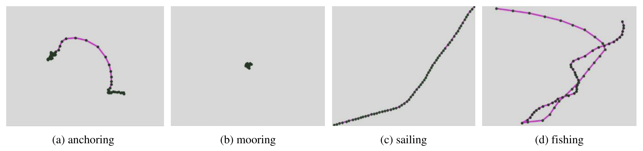
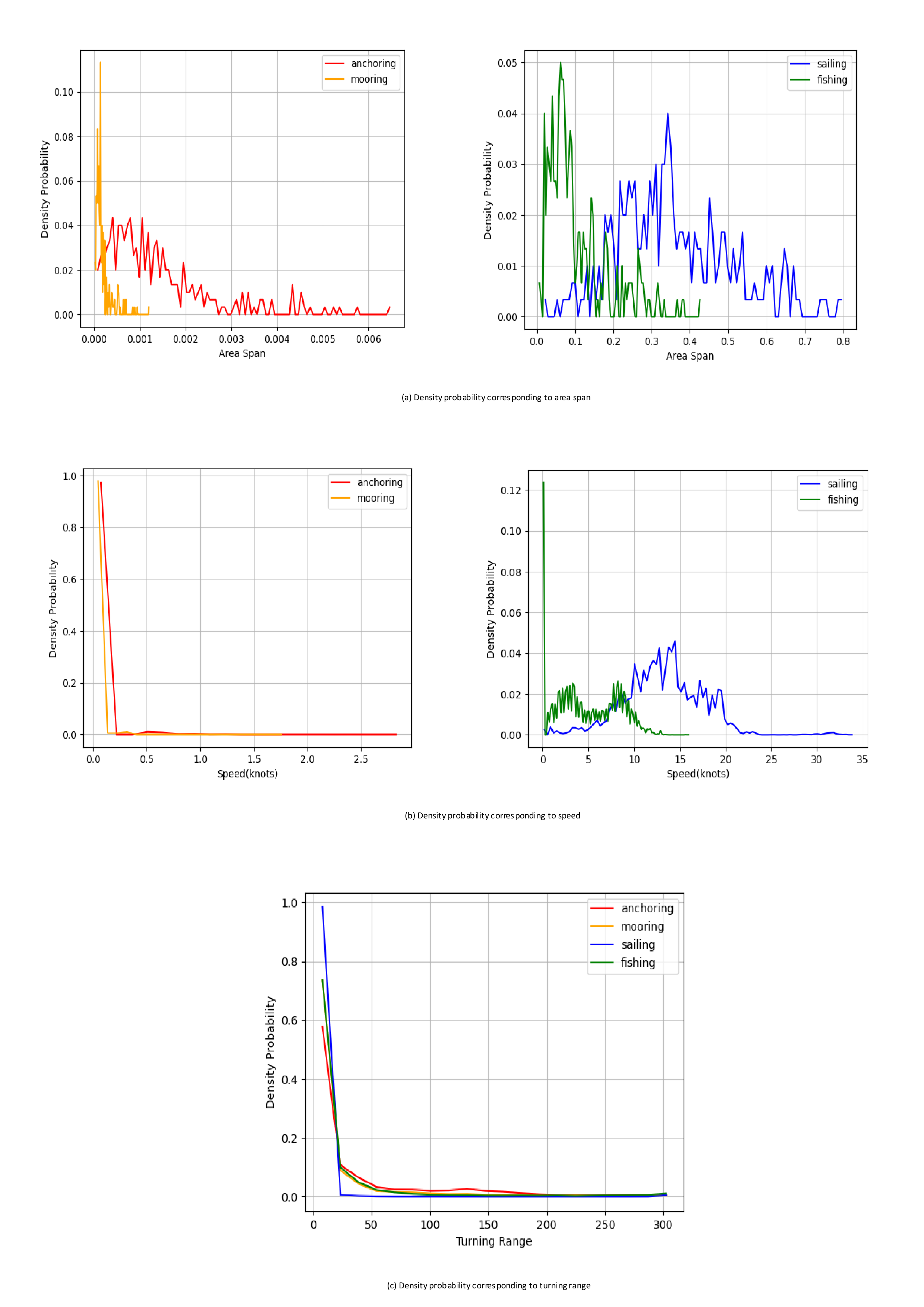
Figure 3 shows the distribution of various characteristics under different behavior modes. This distribution is calculated according to some AIS data collected by the source of the corresponding data set in this article in the past decade. The red solid line represents the anchoring activity, the yellow solid line represents the mooring activity, the blue solid line represents the sailing activity, and the green solid line represents the fishing activity. Since the characteristics of longitude and latitude do not effectively reflect the characteristics of these behaviors alone, the maximum span in the direction of longitude and latitude in the trajectory is introduced here as a regional span for analysis. From Figure 3(a), we can clearly find that the distribution of anchoring and mooring on the regional span is much smaller than that of sailing and fishing. At the same time, the peak of sailing is about 0.34 degrees while the peak of fishing is about 0.6 degrees, which demonstrates that the behavior of fishing usually happens in areas with more fish stocks and a smaller regional span compared to sailing. The regional span of mooring is more limited and concentrated than that of anchoring, which is determined by their different characteristics. In Figure 3(b), we can find that anchoring and mooring show a similar distribution in terms of speed, which is basically below 0.3 knots, and the anchoring has a wider speed range than mooring. The peak of fishing speed is around 0 knots while the peak of sailing is about 14 knots due to the machine break of operation during the fishing process. Figure 3(c) reflects the probability distribution of the change in steering. There seems to be no particularly obvious difference between the four behaviors, however, the steering change of sailing can still be found under careful observation that it is more concentrated in the range below 10 degrees. And there are steering situations greater than 200 degrees in all four behaviors, which is basically in line with the analysis of their characteristics.
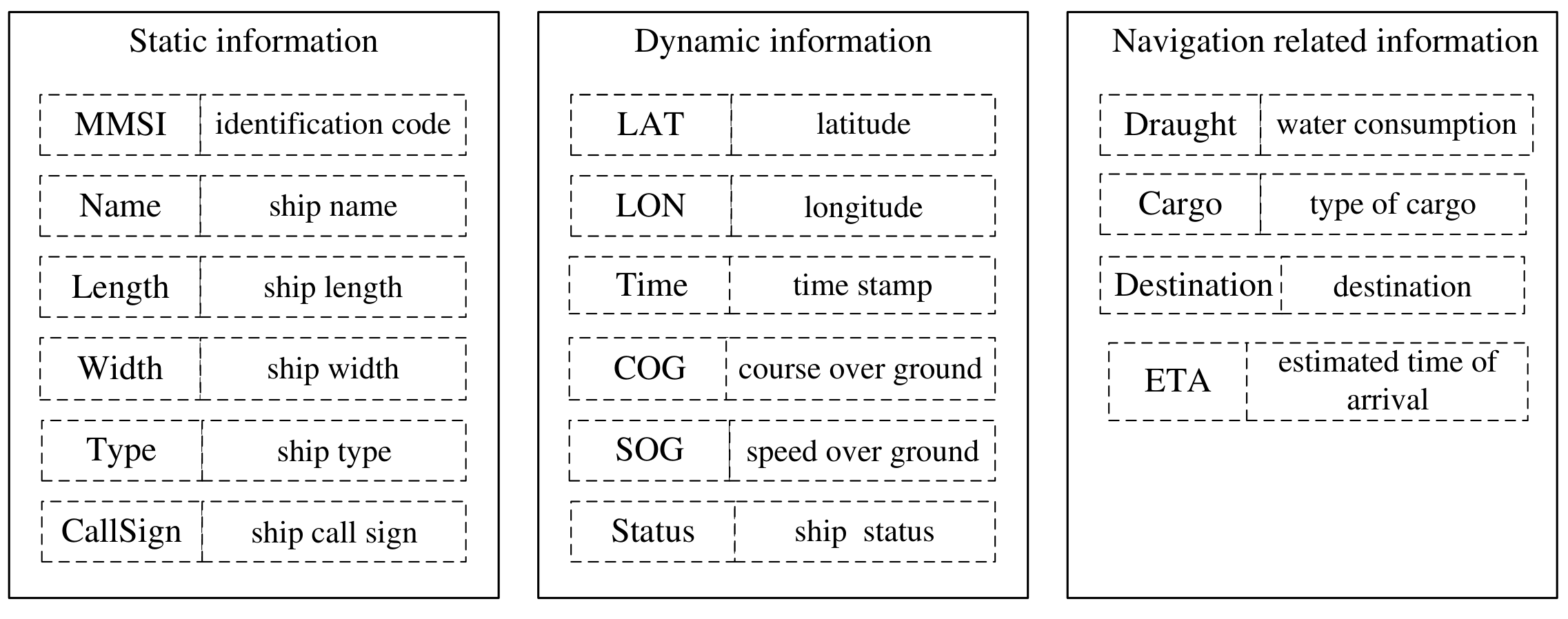
The sources of maritime traffic information are highly varied and include marine radar, base stations and satellites, which use different technologies to monitor and track different ships and vessels. AISs use VHF signals to transmit dynamic, static and navigation-related ship information between ships, satellites and monitoring centers in real time. The main information contained in the transmitted messages is shown in Figure 4. Among them, "Type" refers to the type of the ship itself, such as a passenger ship, or oil tanker, while "Status" refers to the current operation state of the ship, which is also the field to be used later in this paper, such as sailing, fishing, etc.
As the transmission frequency of ship AIS data messages depends on the ship's current speed and the change of its course, the transmission interval is approximately 2 seconds to 3 minutes and is affected by the measurement error of the relevant measurement equipment. When the object moves to a corner or stops suddenly, problems such as position uncertainty and deviation from the trajectory point may arise. In addition, because the navigation state is manually set by the crew, it is prone to errors and can even be manipulated by fishery personnel who tend to hide their operations to conceal illegal acts. At the same time, considering the continuity of ship behavior events in a period of time, we should also consider the effective track that can show its behavior characteristics in this period of time as far as possible. According to the track characteristics of the four behavior modes mentioned in Section 3.1, the generated data set is transformed from the track data to the track image proposed in this paper to help us judge and eliminate obvious errors or invalid label data. For trained deep networks, the input of AIS data with sampling rules, true data and correct labels helps ensure performance and increases their accuracy and stability. Therefore, before being input to the model, the data must be preprocessed using the following steps.
• Feature selection: The AIS dynamic ship information reflects the activity law in ship movement. Therefore, this paper selects a vector composed of longitude, latitude, ground speed and ground course in the dynamic information as the time series data representing the motion of the ship with time.
• Exception handling: Exception handling is conducted for the selected features [11], including null value exception ( in which the value of the selected feature is null), and the direct elimination processing method is adopted; when the change in velocity between the last two data points is greater than the set threshold, the point is considered as an anomalous velocity point and is replaced with the theoretical value calculated assuming that the ship moves with a uniform acceleration in a straight line within this period of time. A similar method is used to address position abnormalities; when the position value of the data point at this time exceeds the elliptical range formed by the data point at the first and second time points as the focus, the point is identified as an abnormal position point is replaced with the midpoint position.
• Data resampling: Considering the relatively slow change in the position of a ship in a marine environment, this paper selects 60 seconds as the unified sampling period; repeated sampling is used to process data points with a sampling interval greater than 60 seconds, and the down sampling method is used for data points with a sampling interval less than 60 seconds.
• Track segmentation: It is generally believed that switching between two modes in a track will often cause rapid changes in direction or speed. Therefore, after resampling the data, we can integrate the changes in the above two attributes and set a threshold to approximately classify different behavior modes in the same track. To maintain the continuous motion characteristics of the trajectory data and account for the real-time performance of the actual application scene, this paper selects a fixed trajectory length of 64 for subdividing the trajectory segments. The navigation status is used as the track category label.
• Normalization: The maximum and minimum normalization method is used to remove the dimensions of the input data, improve the accuracy of the model and increase the convergence speed of the algorithm.
Trajectory image processing is a method for representing the corresponding image of the preprocessed sequential trajectory segment. This paper implements an improved version of SMIGL, originally proposed by Chen et al. [12] to represent the trajectory image. To visualize and effectively classify ship motion modes, three key features (latitude, longitude and ground speed) are captured to characterize the ship motion track modes.
Suppose represents the moving track of a ship, where n represents the length of the track of the number of AIS data points in each track; Vector represents the vector composed of the features contained in the ship AIS data at time , where represents the latitude of the ship at time , represents the longitude at time , represents the ground speed at time ,and represents the ground course at time . The following describes the specific steps for converting each ship track into a corresponding image:
Step 1: Based on the maximum longitude and latitude information of each track, calculate the total horizontal distance and total vertical distance. Then, to better distinguish the anchoring and mooring behavior modes, according to the data distribution of the two behavior modes on the travel distance, determine the corresponding horizontal distance threshold and vertical distance threshold according to the distribution of the travel distance data for the two behavior modes (make sure the track image is in the middle of the picture using the same strategy for the left and right). and represent the maximum and minimum longitudes in Tr, and and represent the maximum and minimum latitudes in Tr. Therefore, the calculation formulas for the corrected total horizontal distance and corrected total vertical distance of the ship are as follows:
Step 2:Calculate the travel distance of each in relative to the minimum longitude and latitude and then obtain the corrected horizontal distance relative to the minimum longitude and the corrected vertical distance relative to the minimum latitude at time . The specific formulas are as follows:
Step 3: According to the above formulas and to the predefined image size (where is 244 in this paper), the percentage of the total distance of each from the respective minimum coordinates in the direction and direction and the exact position of each in the predefined image, respectively, can be calculated to represent the whole track segment in the corresponding image. The specific formulas for calculating the horizontal position and vertical position in the image are as follows:
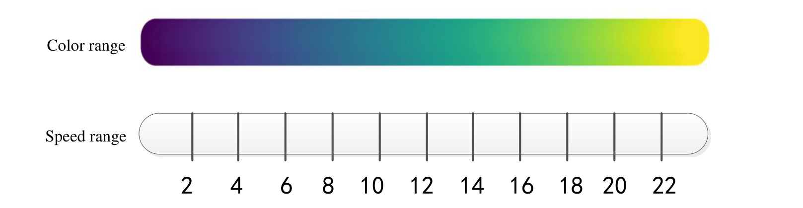
Step 4: After all in are represented in the image of predefined size, considering that each pixel in the image has a corresponding RGB pixel value, each exactly corresponds to one pixel in the image, and the ground speed and RGB pixel value can be represented in a certain range, allowing the ground speed value in each to be mapped to the corresponding RGB pixel value. For example, as shown in Figure 5, the speed relationship between each point is reflected by the size of the pixel values. Finally, the Bresenham line algorithm [13] is used to connect the continuous pixels each time with lines of other colors, thus completing the whole trajectory image processing process.
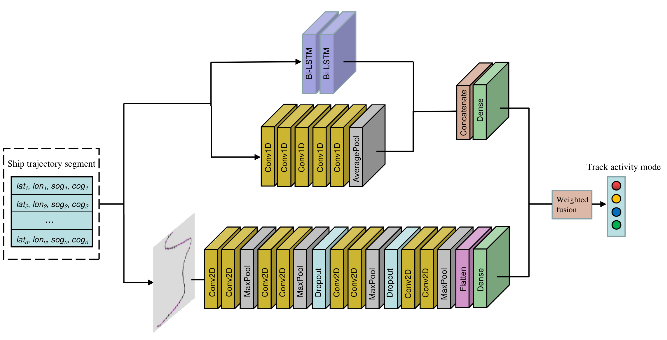
In this paper, a fusion model combining the time-series domain and computer-vision domain is proposed to classify ship trajectory activity patterns.Through the extraction of features from AIS trajectory data from different angles obtained during ship motion, the complementary fusion of two different domain models is used to accurately classify and recognize ship behavior patterns. The specific fusion network model structure is shown in Figure 6.
First, the preprocessed, fixed-length AIS track segment is used as the input to the fusion model. Since the length of the track segment selected in this paper is 64, . The time-series domain model is an improved version of the MLSTM-FCN model proposed by Karim et al. [14] for multivariate time variables. We use two Bi-LSTM layers in the upper branch of the time-series domain model to extract the temporal characteristics and exchange the dimensions of the input multivariable AIS data before it enters the Bi-LSTM layer. N time steps are needed to process M variables (N > M) in each time step before swapping, while only M time steps are needed to process N variables in each time step after the transformation. Experiments show that data dimension exchange first can greatly reduce the training time without reducing model performance. In the lower branch, a fully convolutional network (FCN) consisting of five 1D-CNN layers is used to extract spatial features. Finally, the decision outputs in the time series domain are obtained through feature fusion and dense layers. The computer vision-domain model domain needs to image the ship AIS track segment first, then use the generated track image as the input, extract the features of the track image through multilayer 2D-CNN and MaxPool layers, and use a Dropout layer to improve the generalizability. Finally, the decision output in the computer vision domain is achieved through a dense layer.
After separately obtaining the decision output vectors from the models in the two domains, the final decision output of the domain fusion network is produced through class-weighted fusion [15]. Specifically, once the two decision output vectors are generated, weights are applied, followed by a dot product operation to produce the final output vector. The category with the highest probability in the final vector is the final decision result. Assuming that the output decision vector of the time-series domain model is ,the output decision vector of the computer vision-domain model is , and represents the probability of each ship activity mode (anchoring, mooring, sailing, and fishing ), the results of the decision are as follows:
where is the final decision result and and represent the weight vectors corresponding to the time-series and computer vision-domain decision vectors, respectively. The two weights for each activity mode add to 1, that is, represents anchoring, mooring, sailing, and fishing respectively, and the specific weight values of the weight matrix are determined by subsequent experiments.
To verify the effectiveness of the method proposed in this paper in ship trajectory classification using AIS data, the marine cadastre data source, jointly managed by the Bureau of Ocean Energy Management (BOEM) and the National Oceanic and Atmospheric Administration (NOAA), is adopted. This source contains the navigation records of all AIS-equipped ships along the coast of the United States from 2009 to 2021. In this study, the experimental dataset was constructed by preprocessing AIS data, including 400 trajectory segments per activity category. The dataset was then divided into a training set, validation set, and test set at a ratio of 6:2:2, respectively.
The basic experimental environment used in this paper is introduced in Table 1. Keras is a high-level neural network API, written in pure Python and based on the TensorFlow, Theano and CNTK back-end development libraries. It has a simple deep network programming interface, possessing an easy-to-use API, complete documents and good expansibility. We use Keras to design, debug, evaluate, apply and visualize the deep learning model.
| Hardware/software environment | Detailed information |
|---|---|
| Central Processing Unit (CPU) | Intel Core i7-6800K,3.40GHz,6 core 12 threads |
| Graphics Processor Unit (GPU) | GeForce TITAN X,GDDR5X,12GB |
| Computer Memory | 32 GB,DDR4 |
| Computer System | Ubuntu 16.04, 64 bit |
| Development Framework | Keras 2.3.1 |
| Development Language | Python 3.6 |
Evaluation is an essential step in the experimental process.To evaluate the performance of each experimental model in the experimental process, the feasibility and effectiveness of the model proposed in this paper are verified. The classification evaluation indexes selected in this paper are precision, recall and F1-score. The specific formula is listed below, where TP represents the number of positive classes correctly identified as positive classes, FN represents the number of positive classes incorrectly identified as negative classes, and FP represents the number of negative classes incorrectly identified as positive classes.
The experimental parameters are divided into two parts, each set separately: experimental hyperparameters and network model parameters. In this part of the experiment, the training batch size for each model is 8, the number of iterations is 300, the effective and rapid Adam optimizer is selected, the initial learning rate is set to 1E-3 with decay. After 100 iterations, the learning rate is automatically reduced by to improve model convergence, and the loss function is the classified cross-entropy function. In addition, the class weighting scheme is used to resolve potential class imbalance in the experiment, and the weighting operation of the class factor is used to reduce possible losses in accuracy. The overall hyperparameter settings are shown in Table 2.
| Hyperparameter name | Hyperparameter value |
|---|---|
| Base learning rate | 1E-3 |
| Optimizer | Adam |
| Epoch | 300 |
| Batch size | 8 |
| Loss | Cross entropy |
| Other strategy | Reduce lr, Class weight |
The parameter settings for specific layers of the network model are determined by a controlling variables strategy. The number of memory units (8, 16, 32) and the number of layers (1, 2, 3) of Bi-LSTM are determined through experiments for the upper branch of the time series network, while for the lower branch, experiments are conducted to determine the optimal number of layers (3, 4, 5, 6) and convolution (64, 128, 256, 512) of the 1D-CNN in the FCN. The choice of the network model in the computer-vision domain is mainly based on the trade-off between the accuracy and ability to perform real-time classification of the network. The specific parameters of the double-domain fusion network model are shown in Table 3.
| Layer name | Number,Size | Strategy | Activation |
|---|---|---|---|
| Bi-LSTM_1 | 16,/ | Return sequences=true | Sigmoid |
| Bi-LSTM_2 | 8,/ | / | Sigmoid |
| Conv1D_1 | 256, 8 | Padding=same | ReLU |
| Conv1D_2 | 512, 5 | Padding=same | ReLU |
| Conv1D_3 | 512, 3 | Padding=same | ReLU |
| Conv1D_4 | 512, 3 | Padding=same | ReLU |
| Conv1D_5 | 256, 3 | Padding=same | ReLU |
| GlobalAverage Pool | / | / | / |
| Concatenate | / | / | / |
| Dense_1 | 4,/ | / | Softmax |
| Conv2D_1 | 32, (5,5) | Padding=same | ReLU |
| Conv2D_2 | 64, (5,5) | Padding=same | ReLU |
| MaxPool_1 | /, (4,4) | / | / |
| Conv2D_3 | 128, (5,5) | Padding=same | ReLU |
| Conv2D_4 | 256, (5,5) | Padding=same | ReLU |
| MaxPool_2 | /, (4,4) | / | / |
| Dropout_1 | / | Rate=0.3 | / |
| Conv2D_5 | 128, (5,5) | Padding=same | ReLU |
| Conv2D_6 | 64, (5,5) | Padding=same | ReLU |
| MaxPool_2 | /, (4,4) | / | / |
| Dropout_2 | / | Rate=0.3 | / |
| Conv2D_7 | 32, (3,3) | Padding=same | ReLU |
| Conv2D_8 | 32, (3,3) | Padding=same | ReLU |
| MaxPool_3 | /, (2,2) | / | / |
| Flatten | / | / | / |
| Dens_2 | 4,/ | / | Softmax |
We sought to verify the structural effectiveness and superiority of the model proposed in this paper. First, the effectiveness of the domain fusion model is verified by comparing the double-domain fusion model with the separate domain models. Second, the superiority of the fusion model is verified by comparing it with other representative models that perform similar functions. The comparative experiment is carried out on the same experimental data set, the model is evaluated in terms of the three classification evaluation indexes proposed in this paper, and the optimal performance of the model is obtained through a large number of experiments. Some comparative experimental results are shown in Tables 4 and 5.
| Ship activity class | Precision | Recall | F1-score |
|---|---|---|---|
| Sailing | 97.04±1.26 | 95.37±1.30 | 96.14±1.33 |
| Fishing | 95.50±1.22 | 97.02±1.31 | 96.11±1.41 |
| Anchoring | 64.19±2.47 | 73.64±3.02 | 68.99±2.32 |
| Mooring | 70.21±2.33 | 59.54±2.12 | 64.46±2.20 |
| Accuracy | / | / | 82.00±1.35 |
| Macro avg | 81.89±1.67 | 81.85±1.48 | 82.02±1.22 |
| Weighted avg | 81.89±1.67 | 81.85±1.48 | 82.02±1.22 |
| Ship activity class | Precision | Recall | F1-score |
|---|---|---|---|
| Sailing | 95.28±1.14 | 89.11±0.89 | 92.13±0.97 |
| Fishing | 87.99±1.24 | 95.56±1.10 | 91.59±1.21 |
| Anchoring | 87.19±1.33 | 88.58±1.42 | 87.98±1.27 |
| Mooring | 90.50±0.87 | 87.47±0.86 | 88.95±0.88 |
| Accuracy | / | / | 90.31±0.94 |
| Macro avg | 90.34±1.05 | 90.12±1.13 | 90.14±1.10 |
| Weighted avg | 90.34±1.05 | 90.12±1.13 | 90.14±1.10 |
From a comparison of the above results and the corresponding confusion matrix, the following conclusions can be drawn: (1) For both the time-series model and the computer-vision model, there is a high degree of recognition between the large categories of sailing and fishing and those of anchoring and mooring, because from the perspective of the motion state, the range of position changes and the overall speed range of a ship in the latter categories are significantly different from those of the former. From the perspective of the track images, precisely because of the corresponding performance relationship between them and the motion state, there will be obvious differences among the images. (2) The time-series domain model proposed in this paper performs better in the classification of the sailing and fishing modes because the law of change in the state of motion of ships at sea is obvious when they are in these modes. For example, for a ship in the sailing state, the direction of the ship remains basically unchanged, and the course changes occasionally. However, after a course change, the current course will continue to move forward, and the speed will stabilize within a certain range. In the fishing state, the ship's course and speed will change frequently. They perform slightly worse than track images, which are better at capturing changes in location. (3) The computer vision-domain model proposed in this paper performs significantly better in the classification of anchoring and mooring because there are obvious differences in the trajectory image due to differences in the location range characteristics between the two states. However, for the time-series model, since the course and speed of these two states are also affected by water flow and wind speed, resulting in irregular changes, and the overall changes in position are not as intuitive as images are in the data, it is more difficult to capture the location range characteristics.
The experiments for the fusion model are described below. Because the decision result of the fusion model is the dot product of the weight matrices of the decision results of the two domain models, the choice of weights will also have some influence on the final decision result. Therefore, the following experiments are performed to evaluate the weight factors in the weight matrix separately within [0, 1]; the resulting accuracy of each type of ship activity is obtained as shown in Figure 7.
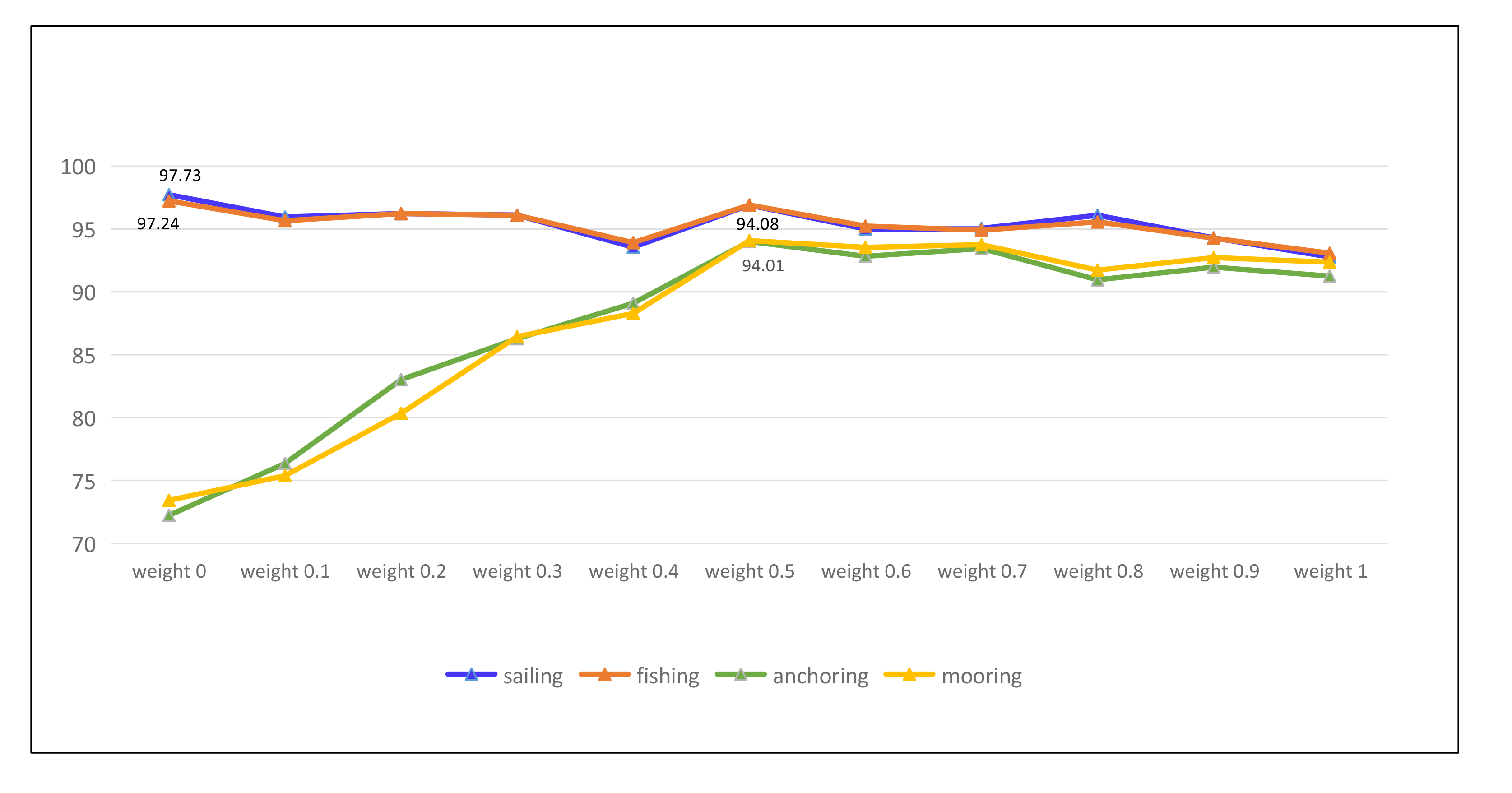
The results show that for both sailing and fishing, as the weight factor in the weight matrix gradually increases, the accuracy decreases slightly at first, then rises slightly, and finally continues to decrease slightly. For both anchoring and mooring, the accuracy increases sharply and then decreases slightly. To obtain the best fusion model recognition result, the weight matrices and are chosen in this experiment. The corresponding weight matrix is applied to the fusion model, and the experimental results are shown in Table 6.
| Ship activity class | Precision | Recall | F1-score |
|---|---|---|---|
| Sailing | 98.79±1.21 | 95.60±1.07 | 97.18±1.12 |
| Fishing | 96.02±0.75 | 99.16±0.84 | 97.57±0.79 |
| Anchoring | 93.76±0.88 | 87.21±1.12 | 90.29±1.08 |
| Mooring | 88.10±0.96 | 94.25±0.75 | 91.16±0.77 |
| Accuracy | / | / | 94.20±0.80 |
| Macro avg | 94.14±0.98 | 94.15±0.85 | 94.17±0.82 |
| Weighted avg | 94.14±0.98 | 94.15±0.85 | 94.17±0.82 |
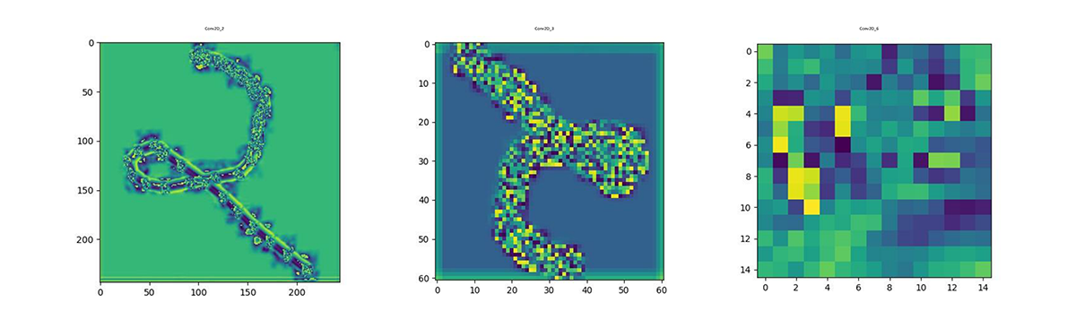
By comparing and analyzing the above experimental results, we find that (1) the overall accuracy of the double-domain fusion model is significantly higher than that of both the single time-series domain model and the single computer vision-domain model. In terms of accuracy for each activity category, the fusion model consistently outperforms the single-domain models, except for the mooring category, where the computer vision-domain model achieves slightly better performance. (2) With regard to recall, the fusion model also demonstrates superior performance across nearly all categories. Notably, it achieves perfect recall for the fishing category, while the computer vision-domain model performs best in the anchoring category. (3) Given the differing trends in accuracy and recall, we further evaluate the models using the F1-score, which provides a balanced assessment. The fusion model achieves higher F1-scores across all categories compared to the individual models, indicating a more robust and consistent classification capability. Fishing behavior records the highest F1-score, while anchoring shows relatively lower performance, though all category scores remain at a high level. Furthermore, feature visualizations of the network layers, as shown in Figure 8, reveal that shallow convolutional layers capture fine-grained details, while deeper layers extract increasingly abstract and high-level representations. These findings collectively confirm the effectiveness and complementarity of the proposed double-domain fusion architecture.
To comprehensively assess the proposed model's effectiveness, we compared it against several state-of-the-art approaches on the same dataset. Karim et al. [14] developed a hybrid architecture combining MLSTM with fully convolutional networks for multivariate time series classification. Arasteh et al. [7] introduced a spatiotemporal feature extraction framework for fishing vessel behavior recognition using AIS trajectory data. Kontopoulos et al. [8] implemented a transfer learning approach based on VGG16 for vessel activity classification by converting trajectories into image representations. Luo et al. [16] proposed a ResNet50-based deep learning model specifically designed for trajectory image classification. The comparative experimental results, presented in Table 7, demonstrate the superior performance of our proposed model across all evaluation metrics.
According to the results of the above comparison experiments, the model proposed in this paper achieves the highest recognition accuracy. For the proposed ship behavior mode task, converting ship track data to track images yields better performance than recognizing ship track data directly as time series data. However, analysis of a ship's trajectory by considering the geometric characteristics of the trajectory is insufficient; the trajectory motion characteristics must also be considered, yielding a better recognition performance and verifying the superiority of the proposed model in performing this task.
In addition, through the analysis of some trajectory data that are not accurately classified by the model, we find that some anchoring states can be easily misidentified as mooring in special environmental situations, for example, the sea surface wind speed and ocean water speed remain within a certain range or even unchanged for a long time in the specified trajectory period, In this special scenario, relevant environmental parameters under the current background need to be added to further distinguish its specific state. Some sailing states will be misidentified as fishing in complex ship intersections or geographical environments. This abnormal adjustment of navigation state caused by external factors will confuse the model to a certain extent. In the follow-up research, if there is corresponding data as support, the ship condition monitoring will be improved more comprehensively by introducing additional environmental parameters and geographical markers into the input parameters of the model.
In this paper, a fusion model combining a time-series domain model and a computer vision-domain model is presented for classifying the four main types of ship motion (anchoring, mooring, sailing and fishing) using AIS data. First, the acquired AIS data are preprocessed, including feature selection, exception handling, data resampling, track segmentation, and normalization processing. Then, the processed AIS data segments are input into a double-domain fusion model network. The upper branch of the time-series domain model captures the characteristics of the attribute data of the AIS data flow resulting from temporal changes, and the lower branch captures the features of the spatial relationship between the attribute data of the AIS data flow. The fusion of the two features is used as the input to obtain the decision vector of the time series domain. In addition, the AIS data segments are processed by track image processing to obtain the corresponding track images as the inputs of the computer vision-domain model, and a corresponding computer vision-domain decision vector is obtained. Finally, through the class weighted fusion strategy, the weighted fusion of the decision vectors from the two domains is selected to achieve accurate classification and recognition of ship behavior patterns. The validity and superiority of the proposed double-domain fusion model in the classification of ship motion tracks are verified by corresponding comparative experiments.
The method proposed in this paper is limited by the size of the network input data, and it has some difficulty in classifying and identifying real-time ship trajectories. In subsequent research, we will attempt to predict ship trajectories to achieve early identification and early warning of ship behaviors. In addition, other, better fusion methods for obtaining the decision vectors can be tested to achieve better classification and recognition results for ship tracks. This will provide solid and reliable technical support for marine regulatory authorities and important scientific and technological support for the realization of a powerful ocean country.
 Copyright © 2024 by the Author(s). Published by Institute of Central Computation and Knowledge. This article is an open access article distributed under the terms and conditions of the Creative Commons Attribution (CC BY) license (https://creativecommons.org/licenses/by/4.0/), which permits use, sharing, adaptation, distribution and reproduction in any medium or format, as long as you give appropriate credit to the original author(s) and the source, provide a link to the Creative Commons licence, and indicate if changes were made.
 Chinese Journal of Information Fusion
ISSN: 2998-3371 (Online) | ISSN: 2998-3363 (Print)
Email: [email protected]

Portico
All published articles are preserved here permanently:
https://www.portico.org/publishers/icck/