A Mimic Fusion Algorithm for Dual Channel Video Based on Possibility Distribution Synthesis Theory

Xiaoming Guo; Fengbao Yang; Linna Ji

doi:10.62762/CJIF.2024.361886

Author's Talk

A Mimic Fusion Algorithm for Dual Channel Video Based on Possibility Distribution Synthesis Theory

Abstract

In response to the current practical fusion requirements for infrared and visible videos, which often involve collaborative fusion of difference feature information, and model cannot dynamically adjust the fusion strategy according to the difference between videos, resulting in poor fusion performance, a mimic fusion algorithm for infrared and visible videos based on the possibility distribution synthesis theory is proposed. Firstly, quantitatively describe the various difference features and their attributes of the region of interest in each frame of the dual channel video sequence, and select the main difference features corresponding to each frame. Secondly, the pearson correlation coefficient is used to measure the correlation between any two features and obtain the feature correlation matrix. Then, based on the similarity measure, the fusion effective degree distribution of each layer variables for different difference features is constructed, and the difference feature distribution is correlated and synthesized based on the possibility distribution synthesis theory. Finally, optimize the select of mimic variables to achieve mimic fusion of infrared and visible videos. The experimental results show that the proposed method achieve significant fusion results in preserving targets and details, and was significantly superior to other single fusion methods in subjective evaluation and objective analysis.

Keywords

image processing

video fusion

mimic fusion

possibility distribution synthesis theory

1. Introduction

Infrared and visible light sensor imaging technologies detect the essential characteristics and differences of scenes and targets through different radiation physical characteristics and detection mechanisms respectively, and there is a great complementarity between the two. Visible video contains texture information that is more suitable for visual perception, while infrared image can capture rich thermal radiation information in low light and other extreme harsh environments. Therefore, dual-channel video fusion can give full play to the complementary advantages of different imaging, reduce data redundancy, and be more conducive to all-weather target detection, tracking and recognition. It has important value in practical applications such as dangerous event monitoring in industrial areas, intelligent obstacle avoidance, medical imaging, and situation awareness [1, 2].

At present, the existing video fusion algorithms can be divided into two categories, static frame-by-frame fusion algorithms and overall fusion algorithms based on spatio-temporal information. Static frame-by-frame fusion algorithms include multi-scale transform fusion algorithms [3], sparse representation fusion algorithms [4], subspace-based methods [5], etc., and their real-time requirements are difficult to guarantee. The overall fusion algorithm based on spatio-temporal information uses spatio-temporal energy matching, spatio-temporal domain structure tensor, high-order SVD and other three-dimensional non-separable transformations [6, 7], and fully considers the spatio-temporal characteristics and temporal characteristics between each frame to ensure the stability and consistency of video data in the temporal domain. Most of the existing dual-channel video fusion algorithms rely on "prior knowledge" to select the fusion strategy. However, in the actual target detection process, due to the dynamics of the detection scene and the variability of the imaging environment, especially the types, amplitudes, frequencies and other characteristics of different features and their changes are more complex. The existing fusion model based on predefined is difficult to adapt to the changes of the "dynamic" difference features. Therefore, the traditional fusion algorithm has become the bottleneck of the performance improvement of the two kinds of video fusion.

In addition, in the current dual-channel video fusion method, most scholars only pay attention to the fusion effect of the algorithm on a single attribute of the difference feature or a single class of the difference feature, but ignore the influence of multiple attributes of the difference feature and the correlation between the features [8, 9] on the selection of the algorithm, resulting in problems such as poor semantic interpretation of the fusion process and difficulty in improving the fusion effect. Therefore, it is very important to study the influence of dynamic changes of multiple attributes such as difference feature types and amplitude between dual-channel videos and the correlation relationship between features on the fusion results for accurate video fusion.

It is found that under different algorithms, the effectiveness of video difference feature fusion has the characteristics of non-probability and interval variation. Generally, it is predicted and estimated based on the fusion strategy of existing and similar scenes, and the possibility distribution has significant advantages in solving the measurement of small sample uncertain information. Distributed composition theory can effectively solve the coordination and combination problem driven by multiple differences. Therefore, this paper proposes a two-way video mimic fusion algorithm based on possibility distribution synthesis theory to solve the problems that the current fusion model cannot adjust the fusion strategy according to the difference information between videos, and lacks of considering the synergy between the difference feature information. The complex relationship between the difference features, fusion strategy and fusion effect is established. It provides a new idea for effectively improving the fusion quality of infrared and visible video [10].

The remainder of this paper is structured as follows. Section 2 presents related work. Section 3 introduces our dual-channel video mimic fusion method. Experiments and discussions are shown in section 4. Subsequently, the conclusion is provided in Section 5.

2. Related Work

Figure 1 Mimic octopus.

Mimicry [11] refers to an ecological adaptation phenomenon in which an organism disguises itself as another organism in terms of behavior, color or morphology, so as to benefit one or both of them. It is the product of long-term evolution of organisms in nature. Multiple mimicry bionics [12] refers to the bionic science that mimics the mechanism and structure of the bionic system based on the study of biological polymorphism characteristics.

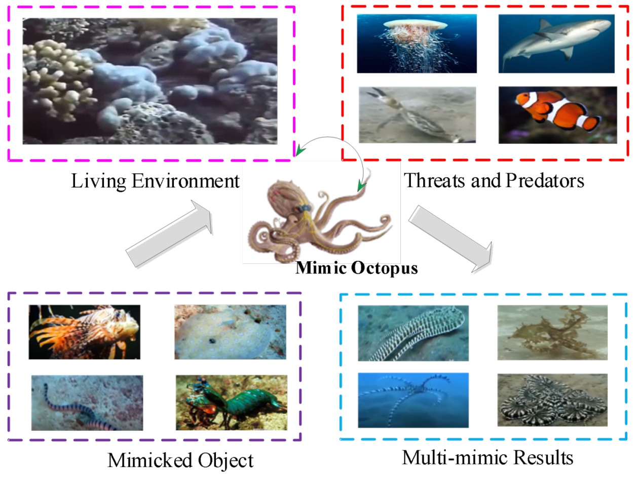
Figure 2 Flow chart of dual channel video mimic fusion method.

Mimic Octopus [13, 14] is a species of Mimic Octopus in the Octopus family, it was first discovered in the waters of Sulawesi Island in Southeast Asia in 1998, the mimetic octopus's anti-sky camouflage function can select the simulated object according to the type of predator it encounters. At present, it can simulate 15 different kinds of creatures such as lionfish, flounder, crinoids, sea snakes, sea anemones, jellyfish, etc., and has super multi-mimicking ability, as shown in Figure 1. For example, when it encounters large predatory fish, it chooses to imitate the venomous creatures of its highly venomous relatives, the blue-ringed octopus, jellyfish and lionfish, to scare off predators. When the mimic octopus disguised as a lionfish and encountered a real lionfish, it immediately switched and disguised as a flounder; when it encountered a flounder, it turned into a sea snake again, when it encountered a real sea snake, it transformed into the surrounding sandy land color, buried itself in the sand directly.

Hu et al. [15] proposed mimic computing by bionic mimic octopus, and developed the world's first mimic computing system aiming at the change and diversity of service objects, which can select and generate multi-functional equivalent computable entities according to dynamic parameters, and also proposed the concept of mimic defense. Gao et al. [16] built a mimic signal processing system based on mimic computing to effectively improve the processing performance and high flexibility of radar signal systems in multiple working modes, aiming at the requirements of high performance, high efficiency and high flexibility of signal processing under the condition of multi-functional integration of distributed opportunistic array radar. Inspired by the imitation ability of the mimic octopus, Xu [17] took advantage of its flexible and bendable advantages to propose a method of segmenting the bionic flexible arm, and established a flexible bionic arm model, which provided an exploration direction for the improvement of the imitation ability of the flexible robot. These methods provide ideas for the difference feature driven fusion in this paper.

Mimic fusion [18] refers to a biomimetic fusion method that imitates the multi-mimic behavior of a variety of organisms according to the survival needs of the mimic octopus, and establishes a variable structure of the fusion model, in order to solve the problem of poor effect or even failure when the fixed model fuses the dynamic scene sequence images, it perceives and extracts the difference features of the corresponding video frames according to the two types of imaging characteristics, and dynamically maps out the optimized fusion algorithm, so that difference features and fusion algorithm are closely combined.

3. Methodology

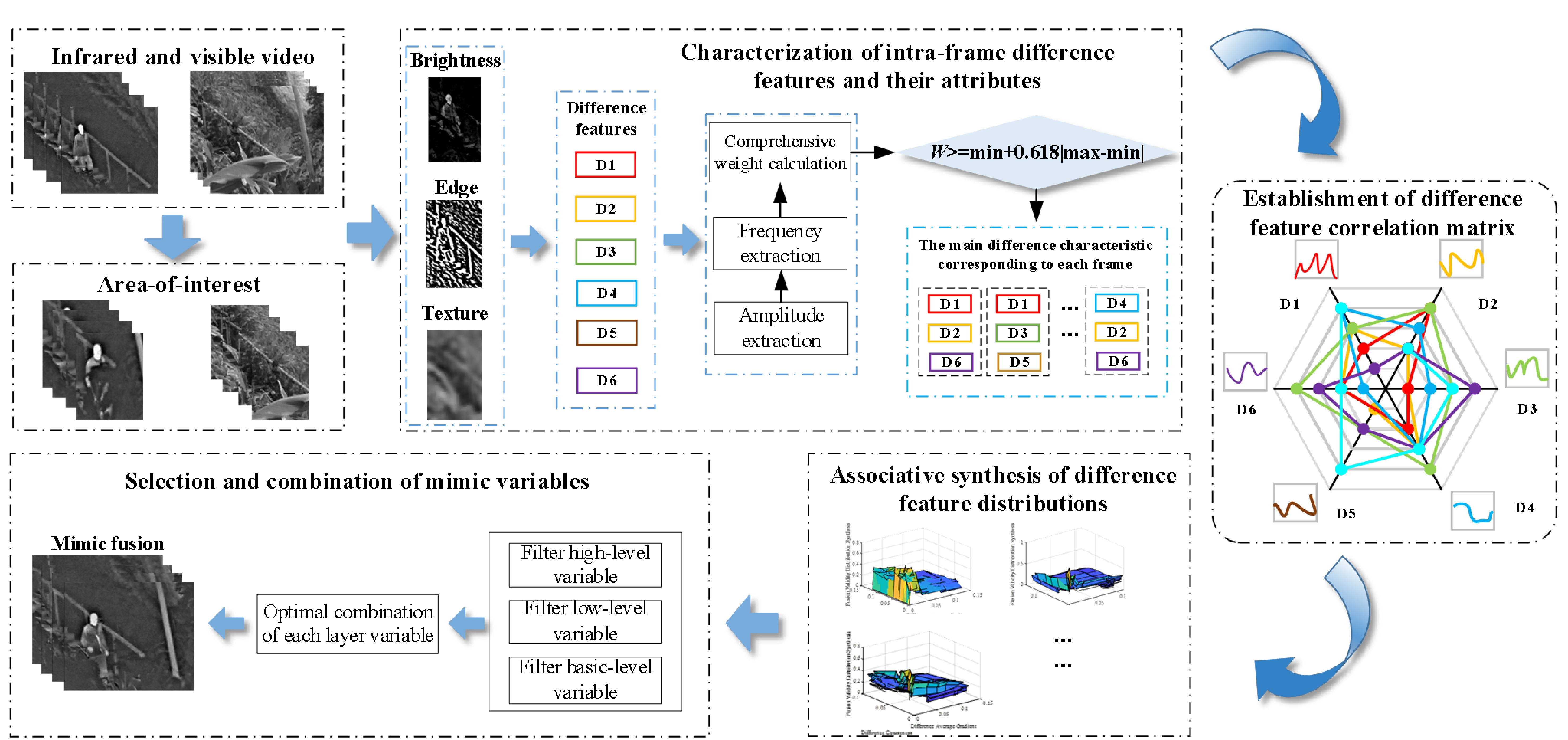
The flow chart of the dual-channel video mimic fusion method based on possibility synthesis theory proposed in this paper is shown in Figure 2, which mainly includes the representation of the difference features and their attributes in the infrared and visible video frames, the establishment of the difference feature correlation matrix, the correlation synthesis of the difference feature distribution, and the selection and combination of the mimic variables. The main process is as follows:

Figure 3 Infrared and visible video frames.

Firstly, the region of interest in the dual-channel video was roughly divided according to the fusion requirements, and six difference features were constructed to quantitatively describe the amplitudes of the three significant types of difference complementary information in the video. The frequency distribution of difference features is obtained using KNN [19, 20], and then the amplitude and frequency of difference features are used to construct comprehensive weights to coordinate the relationship between multiple attributes of difference features. According to the results, the main difference features of each frame are determined. Secondly, the Pearson correlation coefficient was used to measure the correlation between any two different features to obtain the feature correlation matrix. Then, based on the similarity measure, the effective degree distribution of each level variable for different difference features is constructed, and the possibility distribution synthesis rule is used to realize the association synthesis between different class difference feature distributions. Finally, the mimic variables are optimized according to the correlation synthesis results to realize the mimic fusion of the two videos.

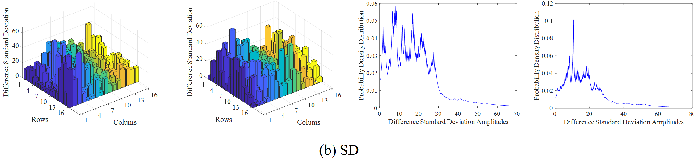
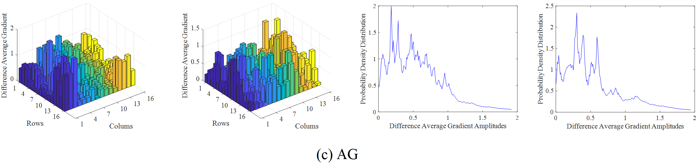
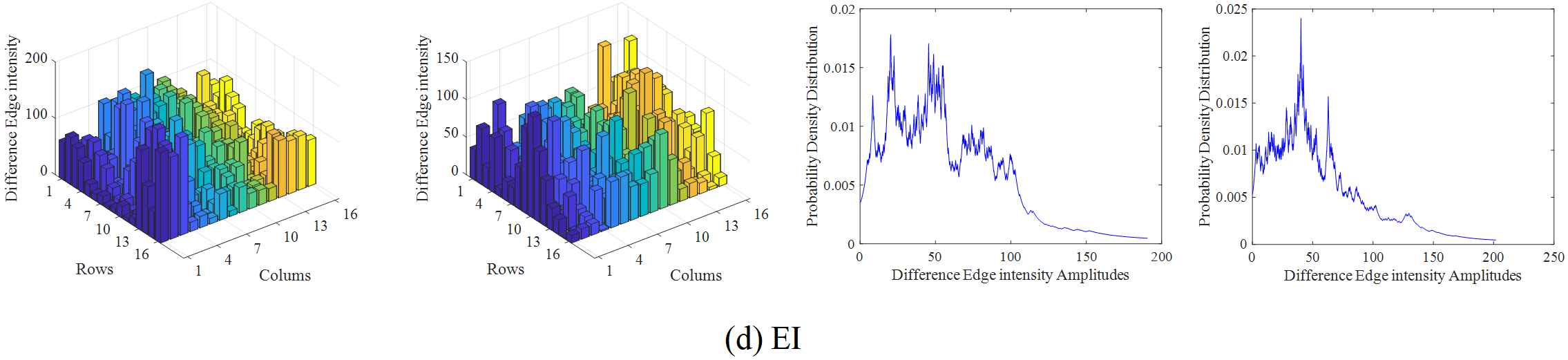
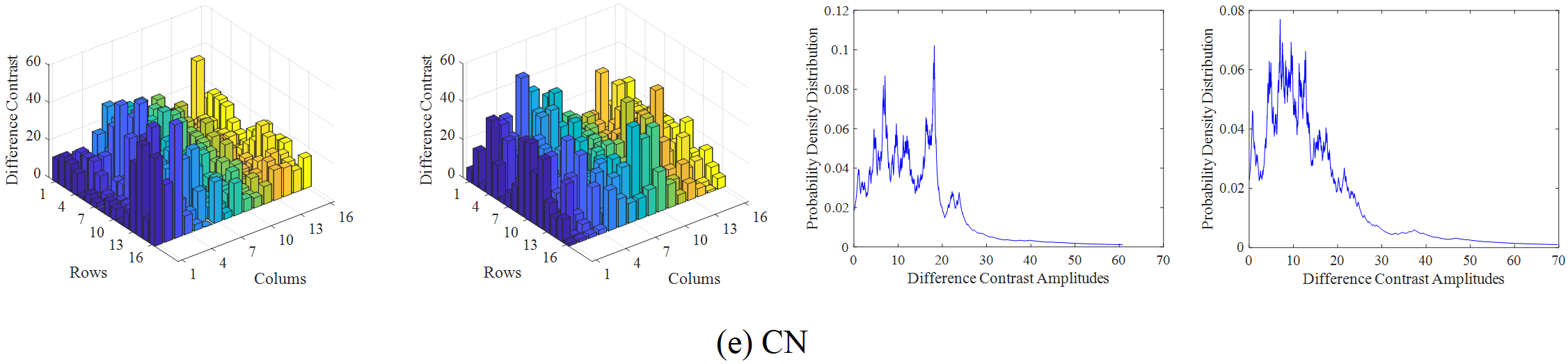
3.1 Representation of intra-frame difference features and their attributes

The main differences between infrared and visible video are in three aspects: brightness, edge, and texture details (as shown in Figure 3). In order to effectively quantify these three types of differences, Mean Gray (GM), Edge Intensity (EI), Standard Deviation (SD), Average Gradient (AG), Coarseness (CA), and Contrast (CN) were used as its representation, and the gray mean was used to quantify the brightness information. Standard deviation, average gradient, and edge intensity are used to represent contrast information, edge clarity, and edge amplitude intensity information of edge information respectively. Contrast and roughness characterize the overall layout of pixel intensity contrast and the roughness of texture information, respectively, and constitute the difference feature set $\{D1,D2,D3,D4,D5,D6\}$ .

The difference feature amplitude $D_{i,r}^{\text{Diff}}$ represents the absolute difference degree of the features in the corresponding frames of the two videos, as shown in Equation (1), $X_{i,r}^{I}$ , $X_{i,r}^{V}$ respectively represent feature amplitude of feature $D_{r}$ to the $i$ th frame for infrared video and visible video.

D_{i,r}^{\text{Diff}}=\left|X_{i,r}^{I}-X_{i,r}^{V}\right|

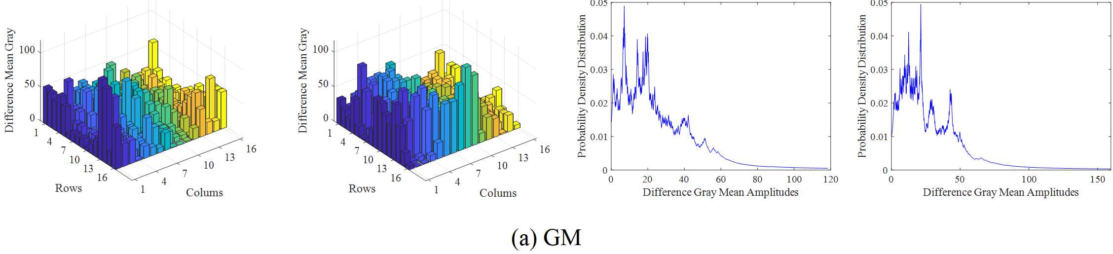
From a macro perspective, the frequency attribute of difference feature reflects the extensiveness of certain difference feature distribution range in the imaging scene, from a microscopic perspective, it reflects the density distribution of a specific feature in the imaging scene with the change of the feature amplitude. Using the K-nearest neighbor nonparametric estimation method (KNN), the probability density distribution of the magnitude of the difference feature can be obtained, thereby obtaining the frequency attribute distribution of the difference feature.

In order to describe the distribution of various feature information of video, we use m⁢n smooth window to perform non-overlapping block processing on the bimodal video sequence frame by frame to extract the corresponding feature information. After the segmentation, the amplitude points of various difference features in each frame of video are all M, which constitute a feature amplitude sample set { $D_{M}$ }. Because the difference feature sample set belongs to small sample information, it is necessary to expand the sample information set to meet the needs of non-parametric probability density estimation. The moving step of $D_{M}$ is set to step, after interpolation expansion, we got { $D_{N}$ }, where $D_{N}^{L}$ is the left boundary of the amplitude sample set, and $D_{N}^{R}$ is the right boundary, Samples $D_{N}^{i}$ are taken arbitrarily from { $D_{N}$ }, so the probability density estimate of difference feature $D_{N}^{i}$ is $p(D_{N}^{i})$ , shown in Equation (2).

p(D_{N}^{i})=\frac{\frac{k_{N}}{N}}{V}=\frac{\frac{k_{N}}{N}}{2\left|D_{N}^{i}% -D_{K_{N}}^{i}\right|}

where

N=\frac{D_{N}^{R}-D_{N}^{L}}{\text{step}},\quad k_{N}=\sqrt{N}

and the probability density value of each amplitude point can be gradually obtained. Using complex trapezoidal integration in each difference feature amplitude sub-interval, approximately obtain the difference feature frequency value $F R$ of each amplitude interval, shown in Equation (3). The amplitude interval $[D_{N}^{L},D_{N}^{R}]$ is divided into $n$ sub-intervals, and each sub-interval $[D^{Lk},D^{Rk}]$ is also divided into the same operation, the step size is set to $h^{\prime}=(D^{R}_{k}-D^{L}_{k})/n$ , and $q$ difference feature amplitude probability density values are included in each sub-interval.

\displaystyle FR=M\int_{D_{L}}^{D_{R}}\left[\sum_{i=1}^{q}p(D_{N}^{i})d(D_{N}^% {i})\right]d(D_{N})

\displaystyle=M\frac{h^{\prime}}{2}\left[p(D^{Lk})+2\sum_{w=1}^{n-1}p(D_{N}^{k% }+wh^{\prime})+p(D^{Rk})\right]

The comprehensive weight of the difference feature is a dynamic function of the proportion of the different attributes of the feature to the whole image, which represents the relative importance of different attributes. As shown in Equation (4), where $\omega(D_{N}^{m})$ is the difference feature comprehensive weight.

\omega(D_{N}^{m})=\frac{p(D_{N}^{m})\cdot D_{N}^{m}-D_{N}^{L}}{D_{N}^{R}-D_{N}% ^{L}}

The main difference feature refers to the fact that for a group of images of different modalities, the difference information of this type of feature is more obvious and prominent than other features, and it is practical feasible and important to use it to guide the late mimic fusion. Since the comprehensive weight of difference features is used to coordinate the relationship between multiple attributes of difference features, its value is more reasonable and apparent comprehensive. In order to accurately judge the main difference features of each frame of dual-mode video, the golden section number is introduced into the comprehensive weight of difference features, and the feature judgment criterion is defined, see Equation (5). Then the main difference features of each frame are determined according to the screening results.

\displaystyle\omega_{i,r}\geq\min(\omega_{i,r=1:k})

\displaystyle\quad+0.618\cdot\left|\max(\omega_{i,r=1:k})-\min(\omega_{i,r=1:k% })\right|

where $\omega_{i,r}$ represents comprehensive weight value of the corresponding feature $D_{r}$ of the $i$ th frame in the video sequence.

Table 1 The calculation formula of

T\otimes

operator.

corr	Correlation of $x, y$	$T\otimes$ operator
$[-1,-0.5)$	Extremely negative correlation	$T_{1}(x\otimes y)=\max(0,x+y-1)$
$[-0.5,0)$	Negative correlation	$T_{2}(x\otimes y)=\max(0,(x^{0.5}+y^{0.5}-1))^{2}$
$[0,0.2)$	Irrelevant	$T_{3}(x\otimes y)=x\times y$
$[0.2,0.4)$	Weak positive correlation	$T_{4}(x\otimes y)=(x^{-0.5}+y^{-0.5}-1)^{-0.5}$
$[0.4,0.6)$	Positive correlation	$T_{5}(x\otimes y)=(x^{1}+y^{1}-1)^{-1}$
$[0.6,1]$	Extremely positive correlation	$T_{6}(x\otimes y)=\min(x,y)$

3.2 Establishment of difference feature correlation matrix and correlation synthesis of feature distribution

Pearson product-moment correlation coefficient (PPMCC) [21], as shown in Equation (6), is used to measure the linear correlation between two variables x and y. Here, it is used to describe the pairwise association relationship between different features. Thus, the feature correlation matrix $\mathbf{T}$ is obtained, as shown in Equation (7), where k represents a total of k kinds of difference feature, $t_{k1}$ represents the correlation value of difference features $D_{k}$ and $D_{1}$ .

\displaystyle\text{corr}(x,y)=\frac{E[(x-\mu_{x})(y-\mu_{y})]}{\sigma_{x}% \sigma_{y}},\,\text{corr}\in(-1,1)

\displaystyle\mathbf{T}=\begin{bmatrix}t_{11}&t_{12}&\cdots&t_{1k}\\ t_{21}&t_{22}&\cdots&t_{2k}\\ \vdots&\vdots&\ddots&\vdots\\ t_{k1}&t_{k2}&\cdots&t_{kk}\end{bmatrix}

Distribution synthesis [22, 23] is to synthesize the distribution of multi-source information according to a certain synthesis rule to obtain a more accurate expression and estimation of information. $\mathbf{T}$ operator is suitable for the case of large intersection of various types of information, and can effectively deal with redundant information. In this paper, the $\mathbf{T}$ operator is used to establish the association synthesis rules of the comprehensive weights of different difference features, and the corresponding synthesis results are obtained. The $\mathbf{T}$ operator is defined as follows:

Let $T\otimes:[0,1]^{2}\rightarrow[0,1]$ be a binary function defined in $[0,1]$ , for $\forall x,y,z\in[0,1]$ , if it satisfies the boundedness,monotonicity, commutative law. The rules are as follows:

\displaystyle(1)\quad T(0\otimes 0)=0,\,T(x\otimes 1)=T(1\otimes x)=x

\displaystyle(2)\quad\text{when }x\leq y,\,T(x\otimes z)\leq T(y\otimes z)

\displaystyle(3)\quad T(x\otimes z)=T(z\otimes x)

\displaystyle(4)\quad T(x\otimes T(y\otimes z))=T(T(x\otimes y)\otimes z)

The feature correlation matrix $\mathbf{T}$ obtained based on Pearson correlation coefficient is combined with the $\mathbf{T}$ operator to obtain the specific calculation formula of the $\mathbf{T}$ operator, as shown in Table 1. That is, according to the obtained correlation matrix element values, the corresponding $\mathbf{T}$ operator is selected for distribution synthesis, so as to establish the difference feature comprehensive weight association synthesis based on multi-rule combination.

By establishing the distribution synthesis between the comprehensive weight of heterogeneous difference features and multiple mimic variables, the projection axis direction of the synthesis distribution is determined by analyzing the importance degree of different attributes of the difference features, so as to obtain the correlation shadow of the fusion effectiveness of multiple mimic variables of heterogeneous difference feature weight function. The fusion effectiveness is to measure the quality of the fusion effect of the mimic variable on a certain difference feature, and the evaluation function of the fusion effectiveness is defined based on the similarity measure, as shown in Equation (8).The larger the value, the more effective the fusion is, and $X_{i,r,\xi}^{F(k)}$ representation of the feature $D_{r}$ of the pixel block $\xi$ corresponding to the fusion result of the $i t h$ frame of the video sequence obtained based on the variable $A_{k}$ .

\displaystyle E_{i,r}^{k}=\frac{1}{N}\sum_{\xi=1}^{N}E_{i,r,\xi}^{k}

\displaystyle=\frac{1}{N}\sum_{\xi=1}^{N}\left(w_{i,r,\xi}^{I}\times\text{SIM}% \left(X_{i,r,\xi}^{F(k)},X_{i,r,\xi}^{I}\right)\right.

\displaystyle\quad+\left.w_{i,r,\xi}^{V}\times\text{SIM}\left(X_{i,r,\xi}^{F(k% )},X_{i,r,\xi}^{V}\right)\right)

\left\{\begin{aligned} \text{SIM}\left(X_{i,r,\xi}^{F(k)},X_{i,r,\xi}^{I}% \right)&=\frac{\sum_{x=1}^{l}X_{i,r,\xi}^{F(k)}(x)\cdot X_{i,r,\xi}^{I}(x)}{% \sqrt{\left(X_{i,r,\xi}^{F(k)}\right)^{2}+\left(X_{i,r,\xi}^{I}\right)^{2}}}\\ \text{SIM}\left(X_{i,r,\xi}^{F(k)},X_{i,r,\xi}^{V}\right)&=\frac{\sum_{x=1}^{l% }X_{i,r,\xi}^{F(k)}(x)\cdot X_{i,r,\xi}^{V}(x)}{\sqrt{\left(X_{i,r,\xi}^{F(k)}% \right)^{2}+\left(X_{i,r,\xi}^{V}\right)^{2}}}\end{aligned}\right.

\left\{\begin{aligned} w_{i,r,\xi}^{I}&=\frac{X_{i,r,\xi}^{I}}{X_{i,r,\xi}^{I}% +X_{i,r,\xi}^{V}}\\ w_{i,r,\xi}^{V}&=\frac{X_{i,r,\xi}^{V}}{X_{i,r,\xi}^{I}+X_{i,r,\xi}^{V}}\end{% aligned}\right.

where $w_{i,r,\xi}^{I}$ and $w_{i,r,\xi}^{V}$ represent the weights of infrared and visible video frames, respectively.

3.3 Selection and combination of mimic variables

Figure 4 Some frames in OTCBVS dataset. From left to right: the 3rd, the 5th, the 9th, the 19th.

Figure 5 Difference feature amplitudes and frequencies.

The mimic variables included in the experiment in this paper refer to high-level variable sets, low-level variable sets and Basic-level variable sets, which are as follows:

High-level variable set: We select seven algorithms in the multi-scale fusion framework, including curvelet transform (CVT) [24], non-subsampling Shearlet transform (NSST) [25], non-subsampling contourlet transform (NSCT) [26], wavelet packet transform (WPT) [27], static wavelet transform (SWT) [28], Laplacian pyramid (LP) [29] and dual-tree complex wavelet transform (DTCWT) [30], which are denoted as $A1-A7$ in turn.

Low-level variable set: The low-level variables in the multi-scale fusion framework were mainly divided into high-frequency rules and low-frequency rules, and the low-frequency rules mainly included simple average weighted (SAW), coefficient maximization (CM), based on window energy (WE). The high-frequency rules mainly include: maximum absolute value of coefficients (MAC), maximum coefficient (MC), based on window energy (WE), where the low and high frequency fusion rules can be arbitrarily combined in pairs [31, 32].

Basic-level variable set: The basic variable in the multi-scale fusion framework of this paper mainly refers to the number of multi-scale decomposition levels and the type of filters in the algorithm. The number of decomposition levels and filters are set according to the algorithm itself.

Based on Equation (8), the mimic variable corresponding to the one with the highest fusion effectiveness is selected as the best mimic variable of the difference feature. The mimic variable with the highest fusion effectiveness and all the mimic variables with the deviation less than 0.05 are considered as the best mimic variable. In addition, the ablation experiment is used in the experiment process, that is, when only the correspondence between the difference features and the high-level variables is studied, the same low-level variables should be used in the fusion process to maintain their consistency. When studying the relationship between difference features and low-level variables and basic-level variables, high-level variables should be fixed.

4. Experiments and discussions

4.1 Source video dataset

Two public data sets are used as examples to demonstrate the rationality of the proposed method. The first dataset is the OTCBVS dataset [33], which contains 17089 different scenes, in which 200 image pairs selected for the experiment are from OSU Color-Thermal change. The second dataset is the TNO Image Fusion dataset [34], which includes multispectral nighttime images related to military phase scenes under different weather conditions, and the Nato_camp_sequence containing 32 image pairs, all 360×270 images, is selected for validation.

Table 2 The main difference feature of each frame.

		The comprehensive weight of the difference feature
Video frame	Discriminant value	GM	SD	AG	EI	CN	CA
3	0.2873	0.2924	0.1895	0.2915	0.2891	0.1492	0.3726
5	0.2758	0.3103	0.2219	0.2739	0.2742	0.1654	0.3431
9	0.2904	0.2234	0.2719	0.3181	0.3078	0.2309	0.3310
19	0.2463	0.1736	0.2632	0.2911	0.2844	0.2350	0.2461

Table 3 Feature association matrix of the 3st frame.

	GM	SD	AG	EI	CA
GM	1.0000	0.1506	0.1485 (T3)	0.1883	-0.1345 (T2)
SD	0.1506	1.0000	0.7439	0.6596	0.0924
AG	0.1485 (T3)	0.7439	1.0000	0.9486	0.0542 (T3)
EI	0.1883	0.6596	0.9486	1.0000	0.0327
CN	0.1551	0.9657	0.6914	0.6152	0.0804
CA	-0.1345 (T2)	0.0924	0.0542 (T3)	0.0327	1.0000

Table 4 Feature association matrix of the 5th frame.

	GM	SD	AG	EI	CA
GM	1.0000	0.2043	0.1629	0.1900	0.0689
SD	0.2043	1.0000	0.7330	0.6997	0.0065
AG	0.1629	0.7330	1.0000	0.9549 (T6)	-0.1628 (T2)
EI	0.1900	0.6997	0.9549 (T6)	1.0000	-0.1897 (T2)
CN	0.2160	0.9690	0.6665	0.6544	0.0197
CA	0.0689	0.0065	-0.1628 (T2)	-0.1897 (T2)	1.0000

Table 5 Feature association matrix of the 19th frame.

	GM	SD	AG	EI	CN	CA
GM	1.0000	0.3681	0.3234	0.3402	0.3726	-0.0558
SD	0.3681	1.0000	0.8470	0.8253	0.9646	0.0921
AG	0.3234	0.8470	1.0000	0.9678	0.8091	0.0201 (T3)
EI	0.3402	0.8253	0.9678	1.0000	0.8098	-0.0446
CN	0.3726	0.9646	0.8091	0.8098	1.0000	0.0716
CA	-0.0558	0.0921	0.0201 (T3)	-0.0446	0.0716	1.0000

4.2 Experimental Cases

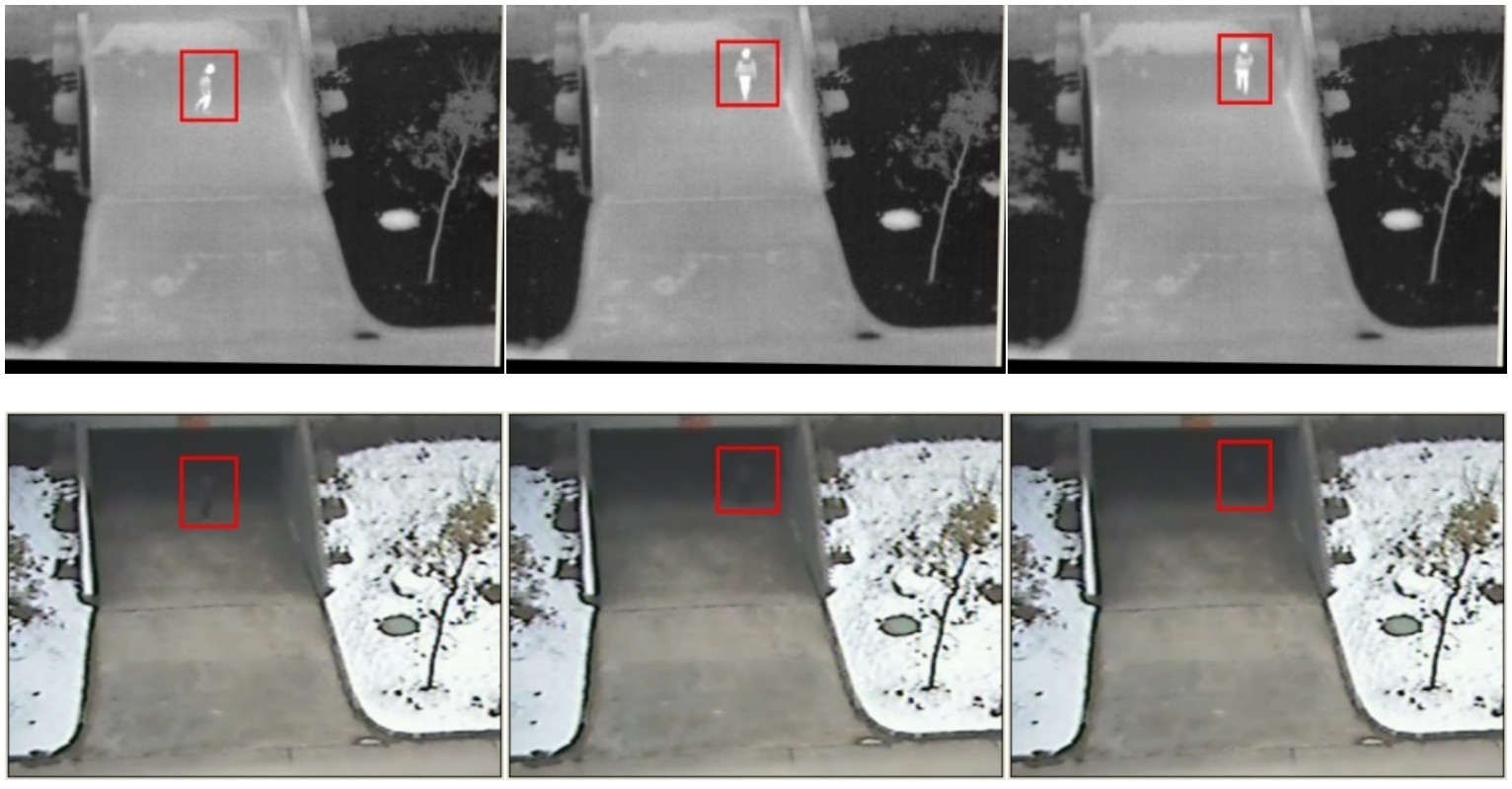
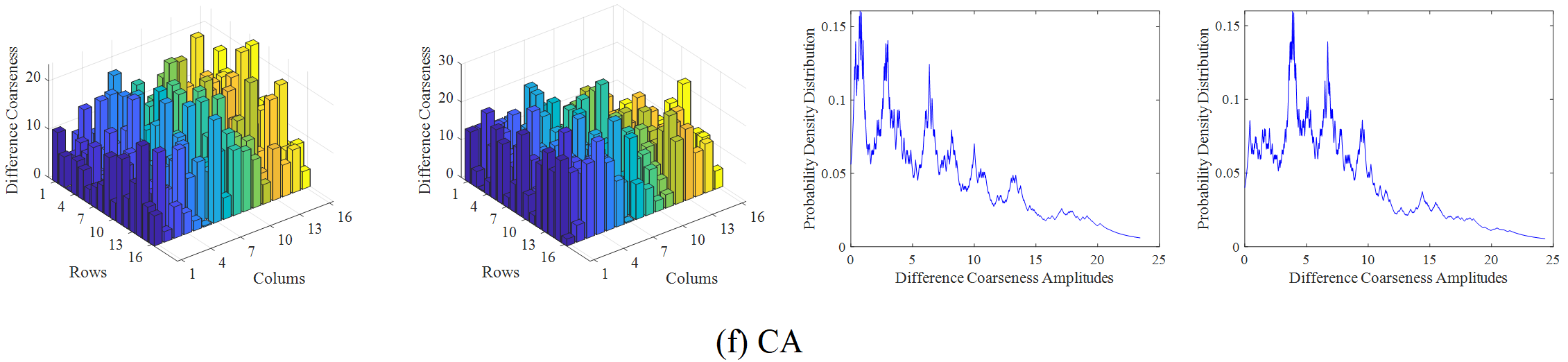
The infrared and visible video selected from the OTCBVS dataset is taken as an example to illustrate the overall process of the proposed method. Firstly, the region of interest is divided, as shown in Figure 4, and then the amplitude of various difference features in each frame of the video sequence is calculated by using formula (1), where m=n=16. Secondly, the probability density distribution of the difference feature amplitude is obtained based on KNN. Here, the step size of the difference feature amplitude point movement is set to, and the sample set is expanded by interpolation, so as to obtain the frequency distribution of the difference feature. The amplitude and frequency distribution results of the difference features are shown in Figure 5.

Calculate the comprehensive weight value of difference features according to Equation (4). For each video frame, the calculated comprehensive weight value of various difference features is filtered and sorted based on the feature discrimination condition, so as to determine the main difference features corresponding to each frame. The results are shown in Table 2, showing the results of frame 3, frame 5, frame 9, and frame 19. The features in red and bold in each row are the main difference features of the frame.

Figure 6 Associative shadow results of difference features for the 3rd frame.

Then, according to PPMCC (see Equation (6)), the correlation relationship between the comprehensive weights of the six types of difference features was calculated respectively, so as to obtain the corresponding feature correlation matrix $\mathbf{T}$ of each frame. The correlation relationship between features was expressed digitally by using table instead of matrix, as shown in Tables 3, 4 and 5. The feature correlation matrix values of frame 3, frame 5 and frame 19 are shown respectively, where the red bold is the main difference feature corresponding to the video frame, which is in one-to-one correspondence with the selected features in Table 3. In addition, the correlation The values between the comprehensive weights of the main difference features in each frame are bold in blue font, and the appropriate $T\otimes$ operator is selected according to the obtained correlation matrix element values, as shown in the brackets in Table 3, the main difference features selected according to the third frame are GM, AG and CA, where $\text{corr}(GM,AG)=0.1485$ , and $\text{corr}(GM,AG)=0.1485$ . $\text{corr}(AG,CA)=0.0542$ , that is, the difference features GM and AG, AG and CA are not correlated, the corresponding T-modulus operator is T3, while $\text{corr}(GM,CA)=-0.1345$ , that is, GM and CA are negatively correlated, T2 operator is selected, and the same is true for other frames.

Finally, the feature fusion effectiveness under different mimic variables was synthesized by pairwise correlation according to the corresponding T-mode operator selected between the main difference features in each previous frame. For the fusion effectiveness synthesis value points corresponding to the comprehensive weights of the two types of difference features, the mimic variable with the largest fusion effectiveness in the mimic variable set was selected by using the disjunction operator. The correlation shadow of the difference feature synthesis results under different mimic variables is established, and then it is mapped to the combination surface of the corresponding two types of difference feature comprehensive weight values.

It is worth noting that if there is only one main difference feature for a video frame, the two steps of calculating the feature correlation matrix and constructing the feature correlation shadow are directly skipped, and the mimic algorithm variables are directly selected through the fusion effectiveness of the difference features under different mimic variables to realize the mimic fusion. If the main difference features of a video frame are $\{f_{a},f_{b},f_{c}\}$ (greater than or equal to two), it is necessary to consider the pairwise association of all elements in the main difference feature set, that is, including $\langle f_{a},f_{b}\rangle$ , $\langle f_{a},f_{c}\rangle$ , $\langle f_{b},f_{c}\rangle$ .

The clusters with the fusion effectiveness of the comprehensive weight function of various difference features in the associated shadow map greater than or equal to 0.1 were divided into significant fusion information areas. The number of occurrences of each mimic variable in the significant fusion information area of the comprehensive weight of various difference features and the corresponding fusion effectiveness value were counted, and the weighted statistics method was used to perform mathematical statistics on the results. Thus, the fusion proportion and average fusion effectiveness of the variable Ai of the mimic algorithm in this region are calculated, and the fusion score index $Fs_{i}$ is constructed, as shown in Equation (11). The fusion score indexes of different mimic variables under the comprehensive weight association method of various differences are summed up, and the mimic variables are determined according to the evaluation, and finally the mimic fusion is realized.

F_{S_{i}}=Pr_{i}*\overline{E}_{i}

Table 6 The fusion score indicators of different algorithm for the 3rd frame.

Feature Association	Index	$A_{1}$	$A_{2}$	$A_{3}$	$A_{4}$	$A_{5}$	$A_{6}$	$A_{7}$
	$Pr_{i}$	0.0186	0	0.0217	0.8168	0.1180	0	0.0248
	$E_{i}$	0.1717	0	0.1668	0.3316	0.1729	0	0.1717
GM and AG	$Fs_{i}$	0.0032	0	0.0036	0.2708	0.0204	0	0.0033
	$Pr_{i}$	0	0	0.0218	0.8836	0.0945	0	0
	$E_{i}$	0	0	0.2468	0.2827	0.1944	0	0
GM and CN	$Fs_{i}$	0	0	0.0054	0.2498	0.0184	0	0
	$Pr_{i}$	0.0258	0	0.0115	0.9026	0.0602	0	0
	$E_{i}$	0.1440	0	0.1359	0.2985	0.2248	0	0
AG and CN	$Fs_{i}$	0.0037	0	0.0016	0.2694	0.0135	0	0
Sum	$Fs_{i}$	0.0069	0	0.0106	0.7901	0.0523	0	0

Table 7 The fusion score indicators of different algorithm for the 5th frame.

Feature Association	Index	$A_{1}$	$A_{2}$	$A_{3}$	$A_{4}$	$A_{5}$	$A_{6}$	$A_{7}$
	$Pr_{i}$	0	0.1191	0	0.2742	0.3795	0.1330	0.0942
	$E_{i}$	0	0.2462	0	0.4331	0.3376	0.3218	0.1979
AG and EI	$Fs_{i}$	0	0.0293	0	0.1188	0.1281	0.0428	0.0186
	$Pr_{i}$	0.0470	0.0043	0	0.0812	0.6154	0.2521	0
	$E_{i}$	0.2763	0.1480	0	0.2191	0.2728	0.2273	0
AG and CA	$Fs_{i}$	0.0130	0.0006	0	0.0178	0.1679	0.0573	0
	$Pr_{i}$	0.7943	0.0348	0	0.1709	0	0	0
	$E_{i}$	0.2172	0.3216	0	0.3976	0	0	0
EI and CA	$Fs_{i}$	0.1725	0.0112	0	0.0679	0	0	0
Sum	$Fs_{i}$	0.1855	0.0412	0	0.2045	0.2960	0.1001	0.0186

Figure 7 Associative shadow results of difference features for the 5th frame.

Figure 8 Associative shadow results of difference features for the 19th frame.

Figure 9 Shows of OTCBVS dataset. (a) The 1st, (b) the 60th, (c) the 75th, from left to right, from top to down, these images are Infrared image, visible image, the results of CVT, DTCWT, LP, NSCT, NSST, SWT, WPT, and Our method.

Table 8 The fusion score indicators of different algorithm for the 19th frame.

Feature Association	Index	$A_{1}$	$A_{2}$	$A_{3}$	$A_{4}$	$A_{5}$	$A_{6}$
	$Pr_{i}$	0.4290	0.0195	0.0334	0.1031	0.3510	0.0641
	$E_{i}$	0.2655	0.3524	0.1604	0.3184	0.3008	0.4372
AG and CA	$Fs_{i}$	0.1139	0.0069	0.0054	0.0328	0.1056	0.0280

Table 9 The experimental results on the OTCBVS dataset.

Source Database	Method	$Q^{\text{AB/F}}$	$Q_{0}$	$Q_{w}$	$Q_{e}$	MI	VIFF	RCF
		Evaluation Index
	CVT	0.4381	0.4954	0.6685	0.2307	2.0139	0.2706	27.4243
	DTCWT	0.3362	0.4283	0.5968	0.2233	1.8850	0.1558	27.0096
	LP	0.3689	0.4630	0.6235	0.2350	2.0329	0.2009	18.4434
	NSCT	0.4004	0.4571	0.6399	0.2390	2.2304	0.1942	18.5130
	NSST	0.4742	0.4879	0.7221	0.2663	2.2226	0.3412	27.4072
	SWT	0.3043	0.4578	0.5569	0.1988	2.1979	0.1876	19.4402
	WPT	0.2911	0.3961	0.5024	0.1518	1.8995	0.1319	18.8553
OTCBVS	Ours	0.4727	0.4899	0.7238	0.2732	2.2318	0.3498	27.5825

Table 10 The experimental results on the TNO dataset.

Source Database	Method	$Q^{\text{AB/F}}$	$Q_{0}$	$Q_{w}$	$Q_{e}$	MI	VIFF	RCF
		Evaluation Index
	CVT	0.3533	0.4755	0.6365	0.1606	1.9663	0.2530	12.1603
	DTCWT	0.3970	0.4389	0.6348	0.1791	1.8331	0.1981	12.6673
	LP	0.3775	0.3037	0.5225	0.1382	1.6262	0.1782	13.4800
	NSCT	0.4785	0.4653	0.6938	0.2105	1.7680	0.2072	13.4329
	NSST	0.4605	0.4076	0.6487	0.2379	1.7639	0.2362	16.7363
	SWT	0.3542	0.4680	0.6368	0.1654	2.0711	0.2718	10.8920
	WPT	0.3267	0.4369	0.5954	0.1544	1.8690	0.2064	11.6804
TNO	Ours	0.5228	0.4980	0.7609	0.2223	1.8563	0.2156	16.7423

Table 11 The average running time of different fusion methods (Unit: second).

Method	OTCBVS	TNO
CVT	2.925	2.333
DTCWT	1.477	1.816
LP	3.101	4.455
NSCT	2.528	2.643
NSST	1.483	1.470
SWT	2.331	2.314
WPT	2.505	2.218
Ours	1.360	1.609

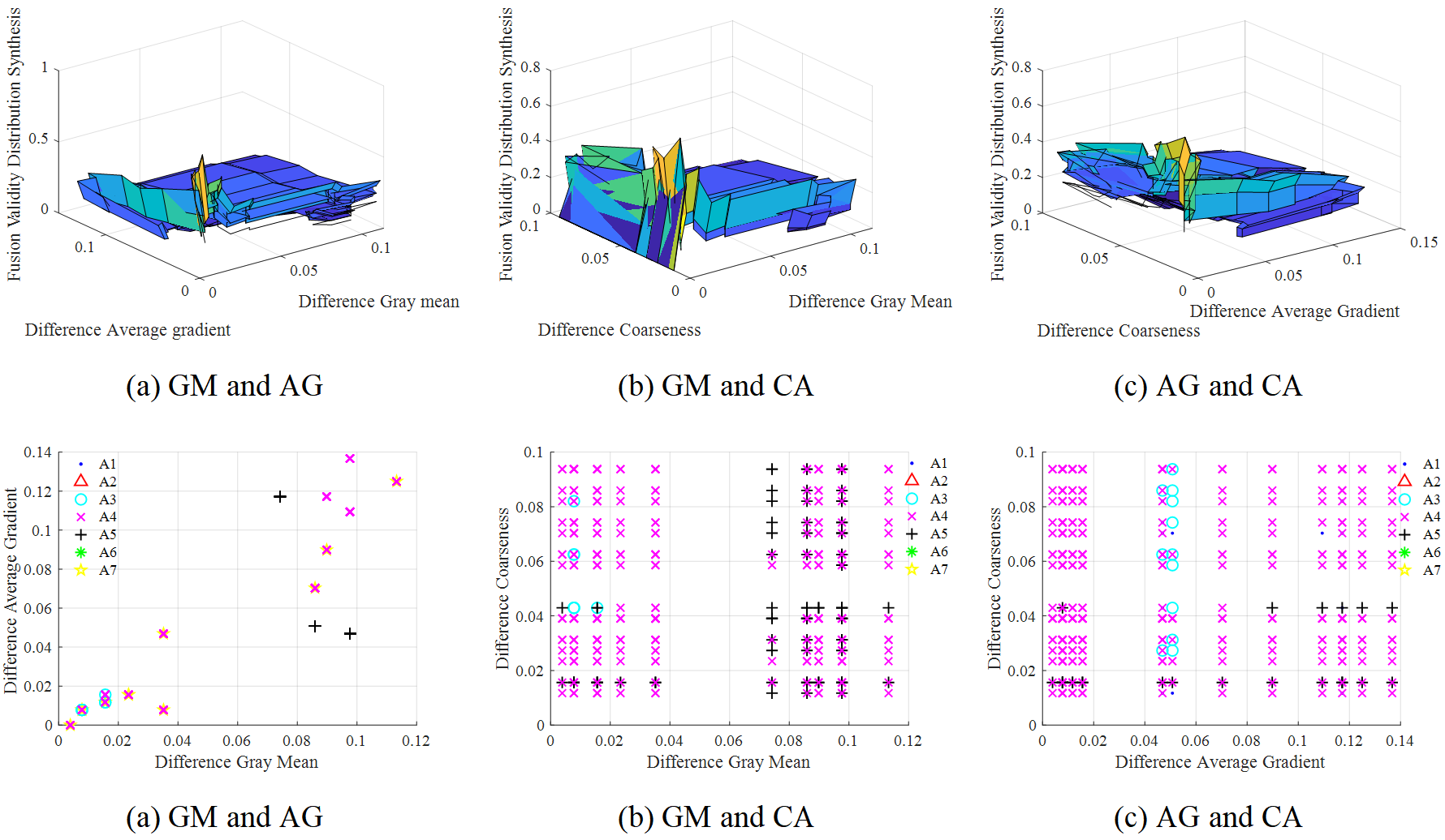
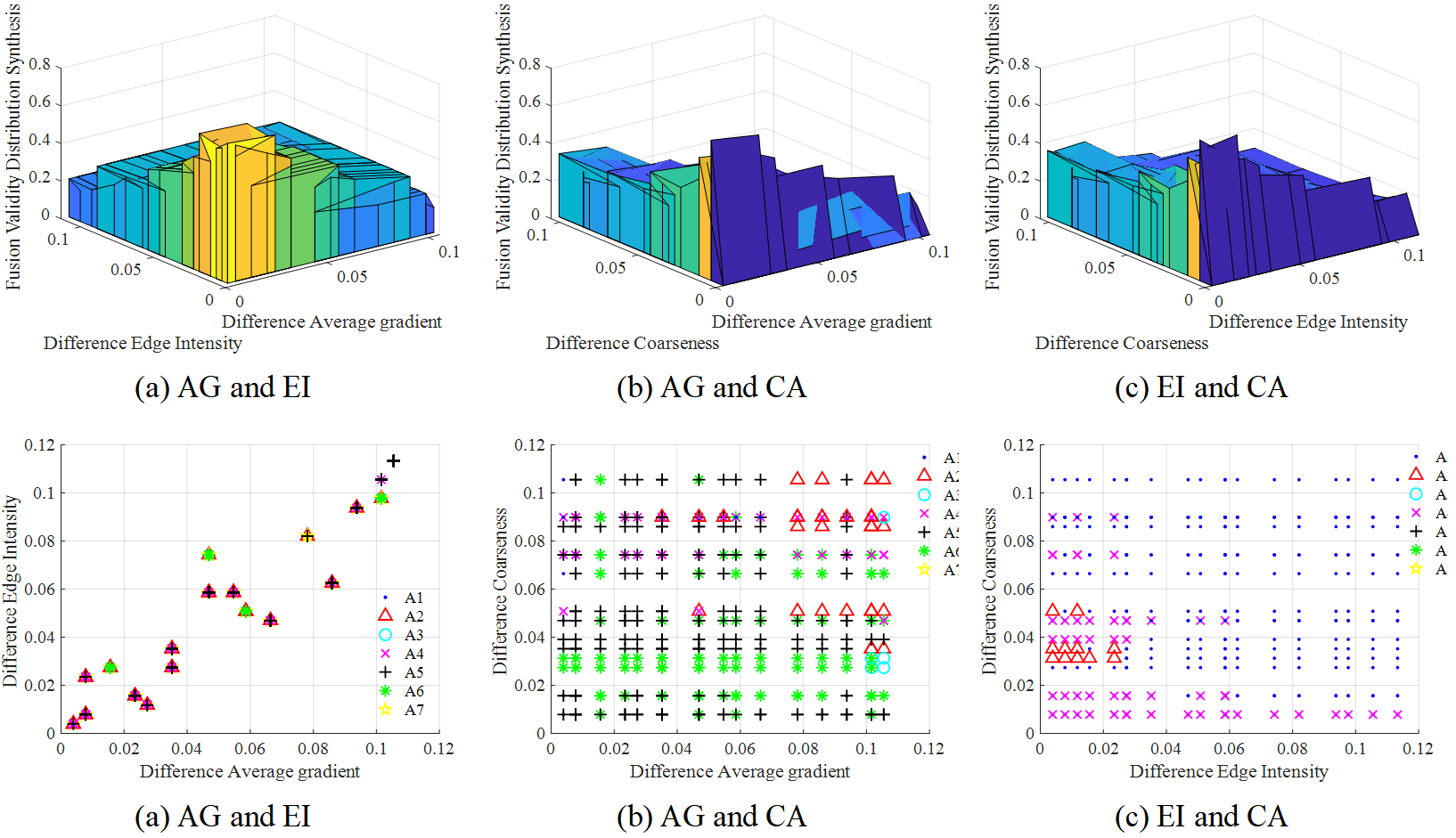
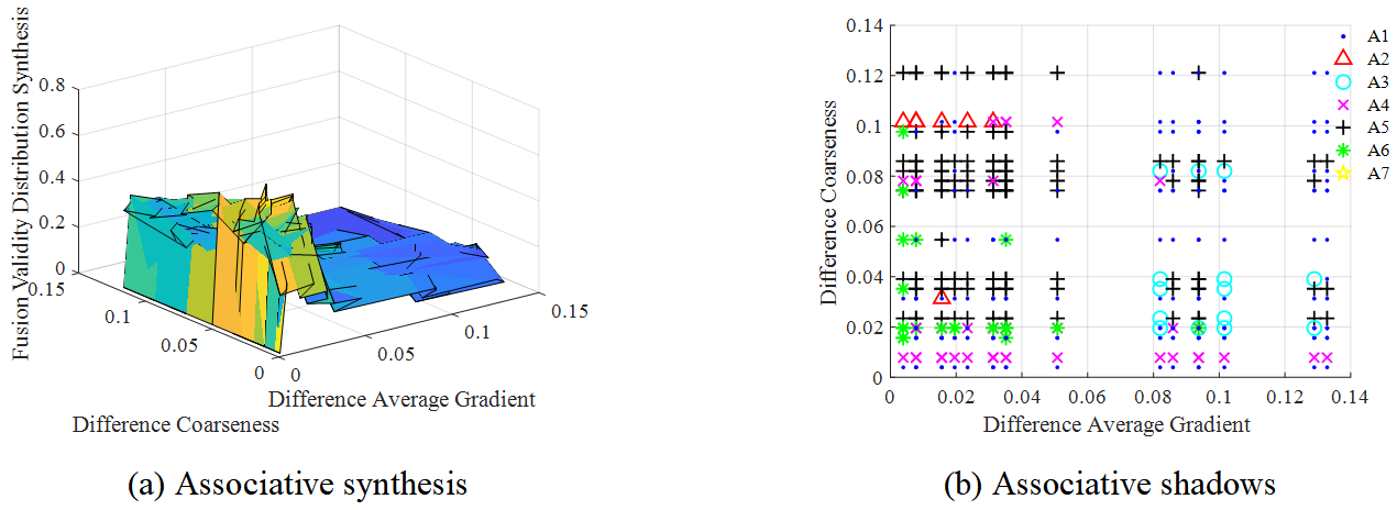
Taking the high-level variables as an example, Figure 6 shows the fusion effectiveness distribution correlation synthesis results of the three main difference features (GM, AG and CA) in the third frame. It is also obvious from Figure 6 that when the weight values of the difference features are equal, the fusion effectiveness points of different high-level variables are relatively densely distributed. That is, the effective information of image fusion is mainly distributed in the part of the associated drop shadow map with smaller comprehensive weight value of features. Table 6 shows the fusion score index values of different algorithms in the three association results, and from the index and size of the last row, it can be concluded that the optimal mimicry high-level variable selected in the first frame is $A_{4}$ . Figure 7 show the feature correlation synthesis and feature correlation shadow results of the three main difference features (AG, EI and CA) in the fifth frame. Based on this, the fusion score index and of various high-level variables are calculated, as detailed in Table 7. $A_{5}$ is selected as the optimal high-level variable to realize mimic fusion. Figure 8 shows the feature association shadow map of frame 19. Since there are only two main difference features in frame 19: AG and CA, there is only one association mode. Combining the results in Table 8 and Figure 8, it is obvious that high-level variable $A_{1}$ is superior to other variables and has better fusion performance, as well as the operation of low-level variables and grassroots variables.

Figure 10 Shows of TNO dataset. From top to down, these images are Infrared image, Visible image, the results of CVT, DTCWT, LP, NSCT, NSST, SWT, WPT, and Our method.

4.3 Analysis of experimental results

In order to verify the rationality and effectiveness of the proposed method, we compare it with some classical fusion algorithms, and the parameter Settings of the fusion algorithm are set according to the reference [35]. At the same time, because the subjective evaluation is easily affected by the individual psychological factors and mental state of the evaluators, there is a certain degree of subjective initiative. Seven objective evaluation indicators [36, 37, 38] are used to evaluate the fusion results of various aspects of the algorithm. These include, $Q^{\text{AB/F}},Q_{0},Q_{w},Q_{e}$ , mutual information (MI), VIFF and Spatial frequency (RCF). The higher the index value, the better the fusion performance. In the experiments, red bold and black bold are used to highlight the optimal and suboptimal values. The experiment platform of this paper is Intel (R) Core (TM) i5-5200U operating system of Windows 11.

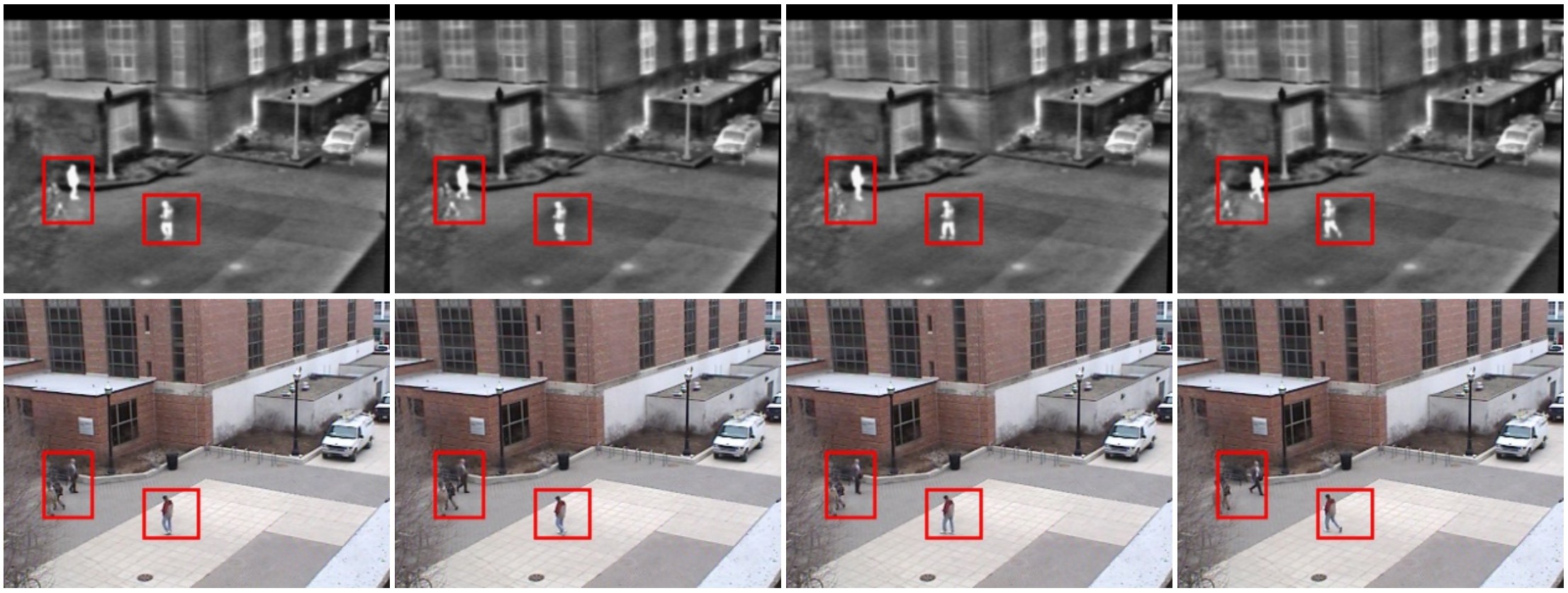
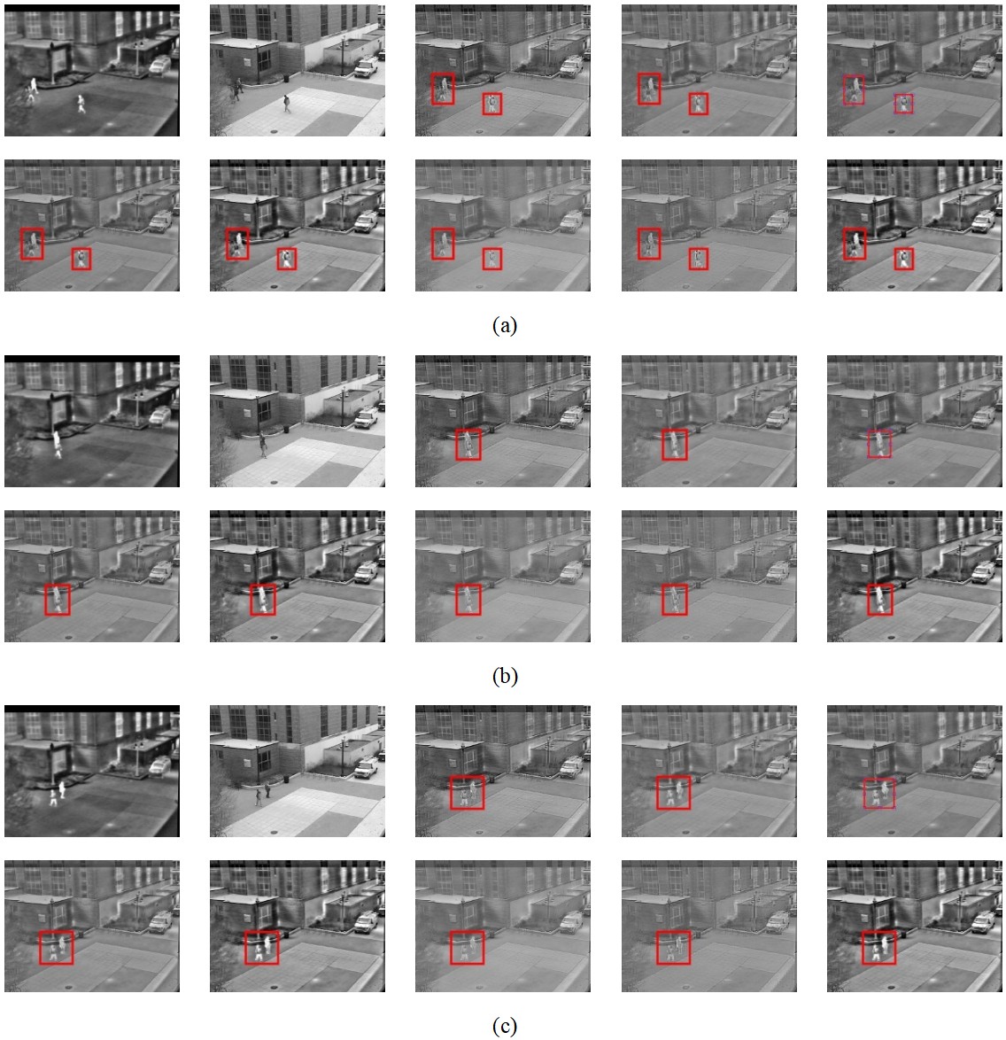
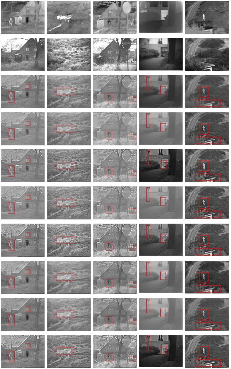
Figure 9 and Figure 10 show the partial fusion results of OTCBVS and TNO datasets respectively. Subjectively, a single fusion algorithm cannot maintain good fusion performance on all data sets. With the change of scene content, the brightness of pedestrians, the edge of buildings and the contour of trees will randomly lose information. On the other hand, the proposed method can better retain the target brightness and detail information, showing stronger intensity distribution, and more realistic and clear texture on moving objects. In the qualitative evaluation of the results, the proposed method has obvious advantages in retaining the details of infrared targets and visible light. Table 9 and Table 10 show the objective quantitative analysis results of OTCBVS and TNO datasets, respectively. In Table 9, the proposed method achieves the best values in $Q_{w},Q_{e},$ MI, VIFF and RCF, and is second only to NSST and CVT in $Q^{\text{AB/F}}$ and $Q_{0}$ . In Table 10, the proposed method achieves the best values in terms of $Q^{\text{AB/F}},Q_{w},Q_{0}$ , and RCF, which is second only to NSST in $Q_{e}$ . It shows that the proposed method contains rich texture information and salient information in the fused image, retains more useful feature information in the source image pair, and has better fusion performance than other methods, which is consistent with the above subjective qualitative evaluation. From Table 11, it is obvious that the proposed method also meets the real-time fusion requirements in terms of time efficiency.

5. Conclusion

In this paper, we propose a mimic fusion algorithm for dual channel video based on possibility distribution synthesis theory, which is inspired by the multi-mimic idea of mimic octopus. Ours method establishes the corresponding set-value relationship between the correlation synthesis distribution of different features and the mimic variables, solves the problem that the existing fusion model cannot dynamically adjust the fusion strategy according to the correlation between the multiple attributes of different features in the video frame and the mimic variables, so as to ensure the full play of the fusion performance. The fusion results of OTCBVS and TNO datasets show that the proposed method retains the typical infrared target and visible structure details as a whole, and the fusion performance is significantly better than other single fusion methods.

Data Availability Statement

Data will be made available on request.

Funding

This work was supported in part by the National Natural Science Foundation of China under Grant 61972363 and Grant 61672472; in part by the Fundamental Research Program of Shanxi Province under Grant 202203021221104.

Conflicts of Interest

The authors declare no conflicts of interest.

Ethical Approval and Consent to Participate

Not applicable.

References

Zhang, M., Dong, L., Ma, D., & Xu, W. (2022). Infrared target detection in marine images with heavy waves via local patch similarity. Infrared Physics & Technology, 125, 104283. https://www.sciencedirect.com/science/article/pii/S135044952200264X
[Google Scholar]
Ma, J., Ma, Y., & Li, C. (2019). Infrared and visible image fusion methods and applications: A survey. Information fusion, 45, 153-178. https://www.sciencedirect.com/science/article/pii/S1566253517307972
[Google Scholar]
Chen, J., Li, X., Luo, L., Mei, X., & Ma, J. (2020). Infrared and visible image fusion based on target-enhanced multiscale transform decomposition. Information Sciences, 508, 64-78. https://www.sciencedirect.com/science/article/pii/S0020025519308163
[Google Scholar]
Li, H., Wu, X. J., & Kittler, J. (2020). MDLatLRR: A novel decomposition method for infrared and visible image fusion. IEEE Transactions on Image Processing, 29, 4733-4746. https://ieeexplore.ieee.org/abstract/document/9018389/
[Google Scholar]
Fu, Z., Wang, X., Xu, J., Zhou, N., & Zhao, Y. (2016). Infrared and visible images fusion based on RPCA and NSCT. Infrared Physics & Technology, 77, 114-123. https://www.sciencedirect.com/science/article/pii/S1350449516300330
[Google Scholar]
Zhang, Q., Wang, Y., Levine, M. D., Yuan, X., & Wang, L. (2015). Multisensor video fusion based on higher order singular value decomposition. Information Fusion, 24, 54-71. https://www.sciencedirect.com/science/article/pii/S1566253514001146
[Google Scholar]
Zhang, Q., Wang, L., Ma, Z., & Li, H. (2012). A novel video fusion framework using surfacelet transform. Optics Communications, 285(13-14), 3032-3041. https://www.sciencedirect.com/science/article/pii/S0030401812002179
[Google Scholar]
Guo, X., Ji, L., & Yang, F. (2021). Dual-mode Infrared Image Fusion Algorithm Selection Based on Possibility Information Quality Synthesis. Acta Photonica Sinica, 50(3), 167. https://www.researching.cn/articles/OJc09b5d2325a67d45
[Google Scholar]
Guo, X., Yang, F., & Ji, L. (2022). MLF: A mimic layered fusion method for infrared and visible video. Infrared Physics & Technology, 126, 104349. https://www.sciencedirect.com/science/article/pii/S1350449522003309
[Google Scholar]
Yang, F. B. (2017). Research on theory and model of mimic fusion between infrared polarization and intensity images. Journal of North University of China (Natural Science Edition), 38(1), 1-8.
[Google Scholar]
Hanlon, R. T., Conroy, L. A., & Forsythe, J. W. (2008). Mimicry and foraging behaviour of two tropical sand-flat octopus species off North Sulawesi, Indonesia. Biological Journal of the Linnean Society, 93(1), 23-38. https://academic.oup.com/biolinnean/article-abstract/93/1/23/2701347
[Google Scholar]
Ishida, T. (2021). A model of octopus epidermis pattern mimicry mechanisms using inverse operation of the Turing reaction model. Plos one, 16(8), e0256025. https://journals.plos.org/plosone/article?id=10.1371/journal.pone.0256025
[Google Scholar]
Hochberg, F. G., Norman, M. D., & Finn, J. (2006). Wunderpus photogenicus n. gen. and sp., a new octopus from the shallow waters of the Indo-Malayan Archipelago (Cephalopoda: Octopodidae). Mount Sinai Journal of Medicine, 73(8). https://www.mapress.com/mr/content/v26/2006f/n3p140.pdf
[Google Scholar]
Tomita, M., & Aoki, S. (2014). Visual Discrimination Learning in the Small Octopus O ctopus ocellatus. Ethology, 120(9), 863-872. https://onlinelibrary.wiley.com/doi/abs/10.1111/eth.12258
[Google Scholar]
Hu, H., Wu, J., Wang, Z., & Cheng, G. (2018). Mimic defense: a designed‐in cybersecurity defense framework. IET Information Security, 12(3), 226-237. https://ietresearch.onlinelibrary.wiley.com/doi/abs/10.1049/iet-ifs.2017.0086
[Google Scholar]
Gao, Y. Z., Wang, J. M., & Lei, Z. Y. (2021). Method of mimicry signal processing for distributed opportunity array radar. Mod. Radar, 43(11), 1-8.
[Google Scholar]
Xu, D. F. (2018). Research on biomimetic Robot inspired by mimicry of octopus, Hangzhou Dianzi University, 1-15.
[Google Scholar]
Guo, X., Yang, F., & Ji, L. (2023). A mimic fusion method based on difference feature association falling shadow for infrared and visible video. Infrared Physics & Technology, 132, 104721. https://www.sciencedirect.com/science/article/pii/S1350449523001792
[Google Scholar]
Mack, Y. P., & Rosenblatt, M. (1979). Multivariate k-nearest neighbor density estimates. Journal of Multivariate Analysis, 9(1), 1-15. https://www.sciencedirect.com/science/article/pii/0047259X79900654
[Google Scholar]
Langrené, N., & Warin, X. (2019). Fast and stable multivariate kernel density estimation by fast sum updating. Journal of Computational and Graphical Statistics, 28(3), 596-608. https://www.tandfonline.com/doi/abs/10.1080/10618600.2018.1549052
[Google Scholar]
Wang, J. (2013). Pearson correlation coefficient. Encyclopedia of systems biology, 1671.
[Google Scholar]
Bouhamed, S. A., Kallel, I. K., Yager, R. R., Bossé, É., & Solaiman, B. (2020). An intelligent quality-based approach to fusing multi-source possibilistic information. Information Fusion, 55, 68-90. https://www.sciencedirect.com/science/article/pii/S1566253519300685
[Google Scholar]
F. Yang, L. Ji, X. Wang, Possibility Theory and Application, Science Press, Beijing, (2019) 41-45.
[Google Scholar]
Ali, F. E., El-Dokany, I. M., Saad, A. A., & Abd El-Samie, F. E. (2010). A curvelet transform approach for the fusion of MR and CT images. Journal of Modern Optics, 57(4), 273-286. https://www.tandfonline.com/doi/abs/10.1080/09500340903541056
[Google Scholar]
Cheng, B., Jin, L., & Li, G. (2018). General fusion method for infrared and visual images via latent low-rank representation and local non-subsampled shearlet transform. Infrared Physics & Technology, 92, 68-77. https://www.sciencedirect.com/science/article/pii/S1350449517308629
[Google Scholar]
LIU, D., ZHOU, D., NIE, R., & HOU, R. (2018). Multi-focus image fusion based on phase congruency motivate pulse coupled neural network-based in NSCT domain. Journal of Computer Applications, 38(10), 3006. http://www.joca.cn/EN/Y2018/V38/I10/3006
[Google Scholar]
Bao, W., & Zhu, X. (2015). A novel remote sensing image fusion approach research based on HSV space and bi-orthogonal wavelet packet transform. Journal of the Indian Society of Remote Sensing, 43, 467-473. https://link.springer.com/article/10.1007/s12524-014-0430-4
[Google Scholar]
Bashir, R., Junejo, R., Qadri, N. N., Fleury, M., & Qadri, M. Y. (2019). SWT and PCA image fusion methods for multi-modal imagery. Multimedia tools and applications, 78, 1235-1263. https://link.springer.com/article/10.1007/s11042-018-6229-5
[Google Scholar]
Du, J., Li, W., Xiao, B., & Nawaz, Q. (2016). Union Laplacian pyramid with multiple features for medical image fusion. Neurocomputing, 194, 326-339. https://www.sciencedirect.com/science/article/pii/S0925231216002940
[Google Scholar]
Aishwarya, N., & Thangammal, C. B. (2018). Visible and infrared image fusion using DTCWT and adaptive combined clustered dictionary. Infrared Physics & Technology, 93, 300-309. https://www.sciencedirect.com/science/article/pii/S1350449518301361
[Google Scholar]
Zhao, R., Liu, L., Kong, X., Jiang, S., & Chen, X. (2019). Multi-scale fusion algorithm of intensity and polarization-difference images based on edge information enhancement. Optical and Quantum Electronics, 51, 1-24. https://link.springer.com/article/10.1007/s11082-019-1899-4
[Google Scholar]
Wang, X., Yin, J., Zhang, K., Li, S., & Yan, J. (2019). Infrared weak-small targets fusion based on latent low-rank representation and DWT. IEEE Access, 7, 112681-112692. https://ieeexplore.ieee.org/abstract/document/8794577/
[Google Scholar]
IEEE OTCBVS WS Series Bench. http://www.cse.ohio-state.edu/OTCBVS-BENCH
[Google Scholar]
Toet, A. TNO Image fusion dataset [J]. Figshare. data, 2014.
[Google Scholar]
Li, S., Yang, B., & Hu, J. (2011). Performance comparison of different multi-resolution transforms for image fusion. Information Fusion, 12(2), 74-84. https://www.sciencedirect.com/science/article/pii/S1566253510000382
[Google Scholar]
Xydeas, C. S., & Petrovic, V. (2000). Objective image fusion performance measure. Electronics letters, 36(4), 308-309. https://citeseerx.ist.psu.edu/document?repid=rep1&type=pdf&doi=4883a68d4eea3ef73908d3b1068faf94a615222b
[Google Scholar]
Wang, Z., & Bovik, A. C. (2002). A universal image quality index. IEEE signal processing letters, 9(3), 81-84. https://ieeexplore.ieee.org/abstract/document/995823/
[Google Scholar]
Piella, G., & Heijmans, H. (2003, September). A new quality metric for image fusion. In Proceedings 2003 international conference on image processing (Cat. No. 03CH37429) (Vol. 3, pp. III-173). IEEE. https://ieeexplore.ieee.org/abstract/document/1247209/
[Google Scholar]

Cite This Article

APA Style

Guo, X., Yang, F., & Ji, L. (2024). A Mimic Fusion Algorithm for Dual Channel Video Based on Possibility Distribution Synthesis Theory. Chinese Journal of Information Fusion, 1(1), 33–49. https://doi.org/10.62762/CJIF.2024.361886

Article Metrics

Citations:

Google Scholar

12

Crossref

11

Scopus

11

Web of Science

11

Publisher's Note

ICCK stays neutral with regard to jurisdictional claims in published maps and institutional affiliations.

Rights and permissions

Copyright © 2024 by the Author(s). Published by Institute of Central Computation and Knowledge. This article is an open access article distributed under the terms and conditions of the Creative Commons Attribution (CC BY) license (https://creativecommons.org/licenses/by/4.0/), which permits use, sharing, adaptation, distribution and reproduction in any medium or format, as long as you give appropriate credit to the original author(s) and the source, provide a link to the Creative Commons licence, and indicate if changes were made.

Table of Content