


Chinese Journal of Information Fusion
ISSN: 2998-3371 (Online) | ISSN: 2998-3363 (Print)
Email: [email protected]

Unit of imaginary number;
Discrete spatial variables for continuous ones respectively;
Discrete spatial frequencies for continuous ones respectively;
Discrete time variables for continuous one ;
Discrete temporal frequency for continuous one ;
Size of Spatial cell, i.e., sampling interval in space;
Frame period of 2D or 1D data, i.e., sampling interval in time;
Maximum speed of interest, known as a prior for a given problem;
Number of space cells along or direction;
Number of data frames, i.e. the length of 2D or 1D signal along ;
OGM or image at instant for continuous case, denoted as well;
OGM or image at instant for discrete case, denoted as well;
Fourier transform of along any number of dimensions.
Efficient perception of and reasoning about environments is still a major challenge for mobile robots operating in dynamic, densely cluttered or highly populated environments [1, 2, 3]. In the context of DAS (Driver Assistance System) [1, 4, 5, 6] or industrial field applications [7, 8], environment perception (or monitoring) usually includes three interleaved tasks, i.e., SLAM (Simultaneous Localization And Mapping) [9, 10], DATMO (Detection And Tracking of Moving Objects) [11] and CTM (Cell Transition Mapping) [12], which have already received a wide attention in the society of mobile robotics.
For the three tasks above, one of the most important things is the fast and reliable extraction of motion information from successive sensor observations. It consists of MOD (Moving Object Detection) even as well as their velocity estimation, which directly affects the performance of localization, mapping, moving object tracking [13]. Furthermore, high level tasks such as path planning, collision avoidance, will be affected by it as well [14]. For example, reasoning on behaviors in DAS requires to separate environment into static and dynamic parts [15, 6]. False negatives (dynamic objects) can lead to serious errors in the resulting maps such as spurious objects or misalignments due to localization errors [16]. On the other side, false positives (static objects) will degrade the performance and computability of tracking module, since the complexity of typical object tracking algorithm increases combinatorially with object number. Meanwhile, MOT (Moving Object Tracking) and CTM can directly benefit from the accurate and timely velocity estimation for moving objects in the dynamic environments.
This paper discuss the problem of extracting motion information from successive sensor observations, including MOD and their velocity estimation. In order to solve this problem effectively, the first thing of all is choosing a suitable representation of dynamic environments. Among all the existing environment representations, OGM (occupancy grid map) proposed by Elfes [17, 18] is the most popular one, which maps the environment as an array of probabilistic cells and easily integrates scans from multiple sensors, even from different type of sensors, for instance, sonar, laser range finder, IR camera [6]. Considering this tractability of OGMs and its wide use in SLAM and DATMO, this paper will take OGMs as inputs, and pay attention on the problem of extracting motion information from successive OGMs.
Almost all research so far on extracting motion information from OGMs have been done under the framework of DATMO. Petrovskaya et al. [11] propose to classify these methods in three categories: Traditional DATMO, Model-based DATMO and Grid-based DATMO. See [11] and the comprehensive survey [19] for more details about DATMO.
In this paper, we focus our attention on the detection of moving grid cells and their velocity estimation, regardless of the tracking problem on object level. According to different ways of understanding motion, we classify those techniques into three categories: Object-Oriented (OO), Cell-Oriented(CO), and OCcupancy-Oriented(OCO).
OO approaches attribute the dynamic changes of successive local OGMs to moving objects. As a result, DATMO are divided into two sub-problems, MOD and MMOT (Multiple Moving Object Tracking) [3, 13, 4]. MOD is to isolate the moving objects in dynamic environments and MMOT is to achieve their state estimation and filter false alarms using typical multiple target tracking algorithms, such as MHT [13, 4] and JPDA [3]. For MOD we are interested in, a consistency based approach, which is based on inconsistencies observed for new data by comparing them with maps constructed by SLAM [13, 4], has often been used. In [3], a time-fading static map is used for consistency detector instead of the static map constructed by SLAM. Another important clue whether the object is moving or not is those moving objects detected in the past. To exploiting this information, a local dynamic grid map is also created to store information about previously detected moving objects in [13, 4]. If an occupied grid cell is near an area that was previously occupied by moving objects, it can be recognized as a potential moving object. There exist at least three drawbacks as follows for OO motion information extraction:
Consistency-based MOD can not effectively detect those slowly moving objects, such as pedestrians on the road, especially in the case of short time interval between consecutive measurements.
Velocity of every cell can not be extracted from OGMs directly, which usually is estimated by subsequent MMOT algorithm or by fusing MOD results with other sensor capable of measuring velocity, such as radar. For example, in [4], the author proposed a generic architecture to solve SLAM and DATMO in dynamic outdoor environments, in which the object detection results were fusing with radar local data and provide the detected objects with their velocities.
The last, perhaps one having most criticisms, is that under the view of OO, MMOT following MOD usually need complex data clustering and association which have combinatorial complexity and whose performance drastically degrade with the number of false alarms of MOD. To suppress the off-road false alarms given by MOD, [20] integrated the road model into their DATMO framework.
Different from the viewpoint of OO, CO methods think that the dynamic changes of local OGMs are caused by the motion of gird cells rather than objects. The most remarkable work in this aspect is so called BOF (Bayesian Occupancy Filter), [1] and [21]. The former (4D-BOF) combines the occupancy grid with probabilistic velocity objects and leads to a four dimensional grid representation. However, the latter (2D-BOF) still uses a 2-dimensional occupancy grid but attaches an associated velocity distribution for every cell. It is obviously found that the 4D-BOF can represent overlapping objects with different velocities, while the 2D-BOF has the advantages to be computationally less demanding [6]. [2] evaluated these BOFs respectively through two experiments, the collision danger estimation for 4D-BOF and the human tracking for 2D-BOF. BOFs provide a Bayesian framework for grid-based monitoring of the dynamic environment. It allows us to extract information of motion cells, containing both occupancy and velocity, only based on the sequences of local OGMs. Furthermore, the complex track association operations is no need, as not existing concepts of objects or tracks in BOF model. Thus it is very suit for those applications in which information on the object level is not concerned. However, for those applications in which object level information is concerned, [22] give an easy way to integrate the 2D-BOF in [23, 1] with FCTA (Fast Clustering and Tracking Algorithm). Because BOF estimates the occupancy and velocity values for both static and dynamic parts of the environment, the subsequent FCTA has a dependency of parameters. In order to solve this problem, [6] integrated a novel real time scheme of MOD into the framework of [22] so that the static parts could be effectively removed from the output of BOF. The MOD in [6] is essentially a consistency-based detector, but it is based on transferring occupancy information between consecutive data grids rather than performing a complete SLAM solution. See [6] for more details about its MOD method.
The key insight of OCO methods is that the dynamic changes of local OGMs are caused by the flowing occupancies in grid cells rather not by the motion of cells themselves. Thus velocity is no longer defined for cells, but for occupancy inside the cell boundaries [5]. Therefore, every occupied cell could have more than one ancestor cell, that is to say, it can be having different velocities simultaneously. Another key fact under the OCO viewpoint is the occupancy preservation, which means the occupancy cannot disappear, unless at the border. From this viewpoint, [5] proposed an improved 2D-BOF, called as BOFUM (BOF Using prior Map). In BOFUM, the prior map information is encapsulated into the reachability matrix and its probability, which describe respectively whether a cell C can be reached from an ancestor cell A, and how the probability of this transition is. BOFUM also uses additional velocity states for dynamic model adaption, which clearly differs in previous approaches [21, 2]. As a result, BOFUM can predict the cell transitions more accurately than those CO methods. Similar to the reachability matrix and its probability in [5], [12] proposed a concept of CTMap (Conditional Transition Map) to model the motion patterns in dynamic environments. However, the transition parameters of CTMap was learned from a temporal signal of occupancy in cells in [12] rather than the method using in [5]. To extract the possible transition, a local neighborhood cross-correlation method was used in [12], which resulted in a large computationally demanding and was constrained with noise in OGMs, such as leaves or hands shaking. Moreover, the cross-correlation method can only give the direction of cell transition, but not give the full information of cell velocity. Nonetheless, it is worth pointing that regarding occupancy in cells as a temporal signal in [12] open a new window for motion information extraction form OGMs. Following this idea and based on the OCO viewpoint, a dual PHD filter was proposed [24], which can separate the dynamic and static cells and estimate the posterior occupancy and its flowing velocity in each cell under the random finite sets filtering framework. It provided the formal and strong way to deal with the OGMs for multiple purposes, such as BOF, CTMap building. However, like the most of RFS filters, the import modeling process according to the application scenario is relatively hard for the engineers.
In this paper, we attempt to propose a different way of extracting motion information from successive OGMs based on a signal transformation, called the keystone transform (KST) , which has been popularly used in the radar signal processing community. For example, [25] employed the KST was used to remove the linear component of the range migration for the moving target in the synthetic aperture radar (SAR) imaging. [26] proposed the fast implementation of KST based on Chirp-Z transform (CZT) in order to overcome the range migration in the long time coherent accumulation for detecting the dim moving targets. Recently, the high order KST were proposed for the above applications in [27][28] and [29] to correct the three order phase migration of the radar echo signal. For extracting the motion information from the OGMs, there exist many similarities to the range migration correction in the radar signal processing, such as focusing or accumulating the moving object with the unknown velocity, and the concepts of range and Doppler in radar signal processing are like the space cell and the velocity in the OGMs. Nevertheless, there also exist several differences with the KST of radar signal processing. One significant difference is that the radar signal in the complex number field and the OGMs is in the real number field. Another important difference is the unknown motion is usually the redial motion along the line of sight of the radar, although it can be high order motion (i.e. with the non-zero acceleration). However, the spatial motion in the OGMs can be one dimensional along the street way, two dimensional along the ground, and three dimensional in the free space. For the ground mobile robotics, we consider one dimensional and two dimensional cases in this paper.
This paper tries to develop a different way of extracting motion information from successive OGMs based on a signal transformation by extending the KST in the radar signal processing community to the 1D and 2D spatial case. The main theoretic idea occurred in our conference paper [30] and this journal article was mainly enlarged from the three aspects, i.e., the more detailed survey, the fast algorithm implementation of 2DS-KST and the experiments for the extended objects. For the sake of integrity, the original point object test results are also kept in this article.
Occupancy grid maps model the environment as an array of cells. Typically, these are layered out in a two-dimensional grid. However, we first discuss the keystone transform for the one dimensional case, which is called as 1DS-KST hereinafter. One reason is that there has a prior straight line constraint with the motion of objects in many applications, for instance, cars moving on the highway or city roads. Detection and estimation the velocity of object moving along straight line themselves have a certain significance for these cases. Another reason is that 1DS-KST, where the concept of fast time is instead by one dimensional spatial grid, has a more direct relationship with KST in radar signal processing. It is helpful to understand the principle of keystone transform, especially for understanding the two dimensional spatial KST introduced in the next section.
For 1DS-KST, the main assumptions are the following:
The velocities for all moving objects are constant during successive frames.
, i.e., .
The sensor is motionless or the motion of it has been compensated by SLAM or other methods.
The first assumption always holds as long as the total length of time window is very short or the amount of velocity change is less than one velocity resolution cell of KST. The second assumption is borrowed from [12], and it is derived from the Nyquist Sampling condition, which ensures the temporal signal of the occupancies in every grid cell are not aliased at a time sampling period . Meanwhile it ensures the spatial continuity of the motion of objects, which is necessary to filter the non-continuous changes of OGMs. In fact, for typical applications and modern sensors, this condition is easy to meet. For example, if the size of grid cell is equal to 2 meters and the time sampling period is equal to 0.1 seconds, the maximum velocity of objects is 10 m/s, which is enough high for most dynamic environment monitoring applications involving pedestrians, industrial robots and vehicles. As for those applications having higher maximal speed, such as automotive application, we can use a larger or smaller in order to avoid objects "jumping over" adjacent cells. As the focus of this paper is to extract the motion information from OGMs, the third assumption is natural and it can make this problem isolated from other problems, such as registration and localization.
Let us first consider the case that there is only one occupied grid cell, called as an ideal point object blow, in the sensor field of view. Assume it is moving at a constant velocity , , and has an initial position , then for any given time instant , the obtained OGM has the following form:
where denote a unit pulse function, which is defined as
And in (1) is the position of this object at time instant , which can be written as
The Discrete Fourier Transform of can be given as follows
Since the signal is a real signal in the case of OGM, always satisfies conjugate symmetry, i.e.,
Therefore, we only concern the non-negative spatial frequency cells, that is, cells of .
To use KST, we need choose a fixed cell of spatial frequency as a reference. In general, the center frequency within the effective bandwidth of signal is chosen for a reference in the application of radar signal processing. For our case of 1D-OGM, we can multiply by a window in the spatial frequency domain, which corresponds to a spatial filtering process and results in a blurred OGM. Without loss of generality, we denote this window as the following:
So can be selected as the reference. Thus (6) can be expressed as
If let , we can get
Now it is the time to consider a temporal variable . During the time interval , we obtained successive OGMs at some discrete time instants. Without loss of generality, we can assume that , that is to say, we obtain many signals at some time instants .
Since the scale factor between and is variable with , the sampling period and total time interval for are both different in terms of . The sampling patterns of and are shown as Figure 1. Notably, the sampling pattern of is like a keystone shape, that's why this corresponding transform is called as KST.
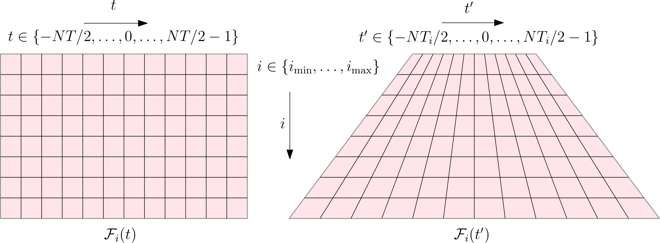
To correct the keystone effect in the sampling pattern of , we need to compute the values at the discrete time for every , which are usually obtained by an interpolate filter in the context of KST. See [31] for more details of the interpolate filter . Thus, after the interpolate filtering,
Then the IDFT transform of in terms of will give the following result:
where is coefficients of spatial filter corresponding with the window .
In general, we must choose an appropriate window type and a suitable width of so that has a locally compact main-lobe and a side-lobe low enough. Thus, for those cells of , the non-zero will not affect the analysis of velocity as long as the distance of object is larger than the width of main-lobe of . This is easy to meet if the moving objects are not closely spaced pixel by pixel. Fortunately, this is the fact in OGM case. In fact, even for the superpositional target, if they have different velocities, the non-zero coefficients of at have no effect to velocity analysis as well. Therefore, let us consider the cell as the next step,
After doing the DFT for in terms of , we can get:
As (19) shown, different velocities will be located at the different frequency grid cells . The KST method, therefore, allow for different velocities in a single cell, which is similar to 4D-BOF [1] and BOFUM [5]. For an object having the velocity , we have the following approximation:
The corresponding resolution of the above velocity measurement is
and the normalized one is
We can choose and according to the dynamic characteristics of environment and the velocity resolution of interest which is related to the minimal detectable velocity.
A one-dimensional OGM is of limited practical use. For mobile robots, the two-dimensional OGM is the usual case. This section will develop a method of two dimensional spatial KST (denoted as 2DS-KST) for the purpose of extracting motion information from successive OGMs. Besides of those assumptions in section 2, two additional ones needed here is as the following:
All objects are moving along nearly the same but unknown direction during frames11.
The unknown motion directions for all objects belong to a prior set with finite number of elements and are constant during frames.
Let us still consider only one ideal point object in the sensor field of view. Assume its initial position is and it has a constant velocity , in which satisfy the condition of . Then for a given time instant , the OGM has the following form:
where denote the region of the cell .
For the 2D spatial case, equation (5) becomes as follows:
where , and .
As the above described, we assume there are finite possible hypotheses for , and denote the th hypothesis as (). But the real case is we don't know the actually moving direction of the object, so we need to do KST for every possible hypothesis, then we can get:
where
, and are projections of vectors , and along the direction, respectively, while is the reference spatial frequency vector for hypothesis when doing KST in next step;
, are projections of vectors , perpendicular to the direction, respectively;
is the two dimensional window function for hypothesis which has the same meaning as the window (8) in one dimensional case.
(4) result from the fact that the item in (3) can be rewritten as:
Furthermore, if the hypothesis is true, that is to say, is approximately parallel to , the last product item in (4) can be ignored further. In this case, for the hypothesis, (4) can be approximated as the following:
where is defined as:
The interpolate filter of Keystone transform is the same as 1D case, so we can get as follows:
The counterpart of the above equation in 1D case is (17). After doing the DFT for in terms of for every occupied grid cell , we can get:
Thus, similar to 1D case, , the magnitude of the velocity in the grid cell can be given as follows:
while the direction of the velocity in this cell is given by , which is the assumption given in the previous, once used in (6).
The velocity measurement given by (11) is in the case of the hypothesis is true for this cell. In practice, we don't know which hypothesis is true for any occupied grid cell in advance, so we must merge the results of those multiple hypotheses so that the correct motion information can be given.
In fact, by 2DS-KST with multi-hypothesis, we can get cuboid , which is the general form of (10) for any arbitrary grid cell under the hypothesis . That is to say, we get the two dimensional matrix for every grid cell , which represents the possible velocity in this cell, including the magnitude (denoted by , which can be negative) and the direction (denoted by ).
Here we use a MPD (Maximal Power Detector) based method for the purpose of extracting the motion information from , which is based on the fact that the power item will be larger when and are more matched with the true value of the velocity. It can be described as the following four steps:
The first step is the maximal merging step:
The second is the following power detector:
The third is the following estimator if holds on:
The last step is the separator as follows:
As the above MPD approach of merging multiple hypotheses only outputs the most likely point estimation for the velocity, it is obvious that it is only appropriate for the case when the occupancies in each grid cell only have one significant velocity during the time interval. Nevertheless, it does not affect the versatility of 2D-KST for extracting motion information. For instance, we can use the more complex GMM (Gaussian Mixture Model) instead of the point estimation in MPD method as the velocity model of occupancy, which would undoubtedly increase the robustness and the compatibility to the complex situations. In fact, which velocity model should be selected is a key problem in practice and it closely depends on the physical application.
For the more complex method of merging multiple hypotheses, it is already beyond the scope of this paper and may be an appropriate topic for the future work.
In the previous two sections, 1DS-KST and 2DS-KST are presented, which are both interpolate filter based KST. In this section, a different implementation of 2DS-KST, which is more effective for our problem, is presented . The other issues related to implementation will be also discussed.
According to the description in Section 3.2, in order to extract the motion information from OGMs, we need the cuboid of under each hypothesis (), rather than the direct result of the keystone transform for the original input . In the previous two sections, we used the interpolate filter based keystone transform to obtain first, then obtained by doing the DFT transform for in terms of .
Here we introduce another implementation without using interpolate filter, which is based on the so called CZT (Chirp-Z Transform)[32]. It can both correct the keystone effect in the sampling pattern of the data and transform them to the domain simultaneously. That is to say, it outputs instead of in the interpolate filter based method, so it is more effective for our problem. More importantly, CZT has the fast implementation and can flexibly control the frequency range to be analyzed. See [32, 26] for more details and applications of CZT. The flow diagram of CZT based 2D-KST is shown in Figure 2, where the data pattern in every step is explicitly shown and the meanings of those variables can be seen in section 2, 3 and the notations before the introduction.
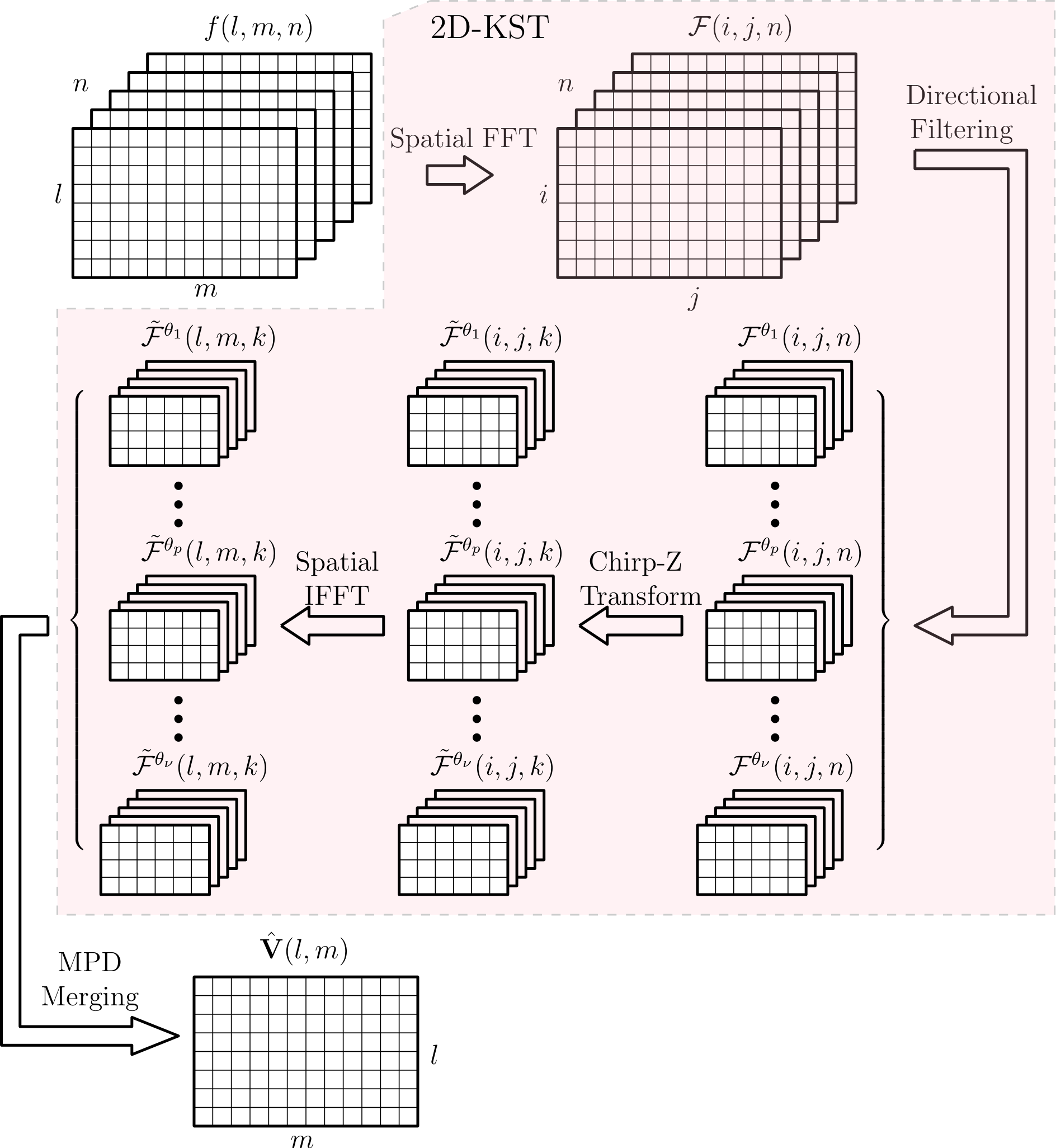
The main steps in Figure 2 are explained as follows:
Spatial FFT: The OGMs are transformed from the spatial domain to the spatial frequency domain by 2D-FFT in this step, which can be done sequentially for each new OGM, or with batch processing for all OGMs through parallel computing. In order to use FFT, is usually a power of . If it is not this case, we can pad zeros at the tail. Thus the complexity of this step is , where ranges around the interval from 4 to 5 depending on the implementation [33].
Directional filtering: The window in spatial frequency domain under every possible direction of velocity is multiplied respectively to the previous results, which corresponds to let every OGM pass several bandpass spatial filters, respectively. Here we use the following rectangle window,
Chirp-Z transform: As described before and shown in Figure 2, CZT is used both to correct the keystone effect in the sampling pattern of the data and to transform them to the domain simultaneously. For our application, the parameters of CZT are set as follows:
Spatial IFFT: As shown in Figure 2, this step uses the 2D-FFT to transform every cuboid from spatial frequency domain to spatial domain. As the migration across grid cells caused by motion has been compensated, the moving grid cell can be focused to the average, initial, or last position during the interval, which depends on the definition of the time index used in the CZT. Obviously, the complexity of this step is .
MPD merging: The velocity of any cell identified as moving one is estimated in this step. The complexity of this step is approximately .
According to the above analysis, the total complexity of 2D-KST can be approximated as follows:
(7) means that the computational complexity of the total processing of 2D-KST is about times more than the complexity of 2D-FFT with the side length .
In this section, we design three experiments to evaluate the performance of the proposed method on the extraction of motion information. The first two is based on numerical simulation data, and the last one is based on the real data from mobile robot.
The first experiment, called as point object test, is to demonstrate the validity of our method through point object data, which means all objects only occupy one grid cell in this experiment. Some intermediate results are also shown as figures in this experiment, which is benefit to understanding the process of KST.
The second experiment, i.e. extent object test, is to illustrate the responses of the spatial frequency window to the different size of objects. Some useful guidelines about how to choose the appropriate parameters for the spatial frequency window are derived further.
The third experiment, referred to as real data test, is to uncover some potential applications for the methods proposed in this paper. Two datasets are used in this experiment, which are collected by the robot in the indoor and outdoor environments respectively. The difference is that the ground truth is known precisely for the first dataset, while it is not the case of the outdoor dataset.
In this experiment, we use the simulation data of point object to test the 1D-KST and 2D-KST. Considering the sensor noise and the imperfections in the OGM building process, we add to the OGMs some Poisson noise, which is uniformly distributed in the grid cells and whose number obeys the Poisson distribution. The main parameters in the simulation is shown in the Table 1, where the velocities are represented in the normalized format, and the scale factor in is defined as follows:
| Parm. | 1D case | 2D case | |
|---|---|---|---|
| OGMs | 128 | 64 | |
| 100 | 40 | ||
| Objects | #0 | ||
| State | #1 | ||
| #2 | |||
| #3 | |||
| #4 | |||
| #5 | — | ||
| Poisson Rate | 16 | 64 | |
| Windows | — | ||
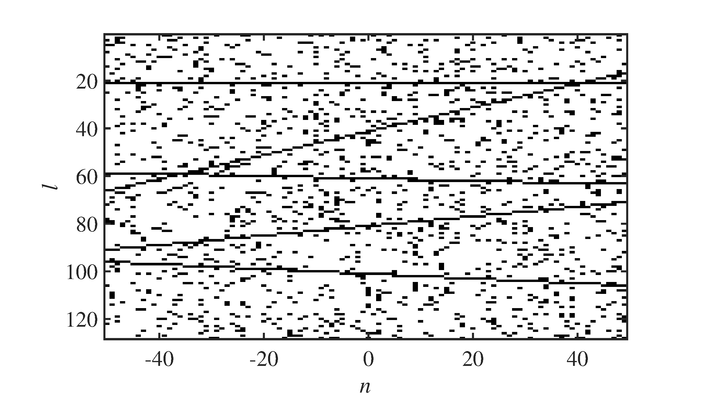
The results of the one dimensional test are shown in Figures 3 - 5. From Figure 3, we can see five objects moving at different speeds along positive direction or negative direction. The speed of the fastest one is , which is the maximal feasible velocity given by the Nyquist sampling theorem, and the speed of the slowest moving object is , which is very close to the velocity resolution given by (22). Through this setting, we can validate 1D-KST in terms of velocity measurement capability. Meanwhile, we set a stationary object at , which can be used to check the performance on the separation of the dynamic grids from the static ones. After adding the Poisson noise, the OGMs look very noisy.
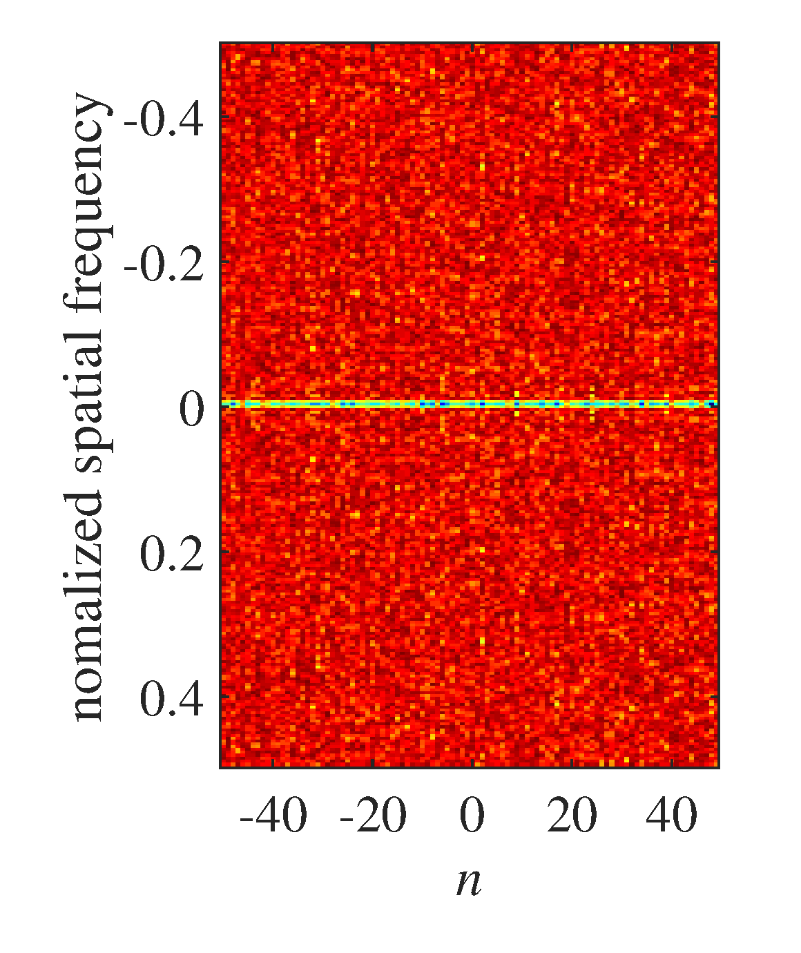
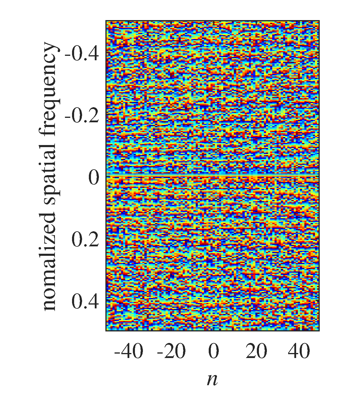
The result of OGM sequence by the spatial Fourier transform is shown in Figure 4. As the noise in the OGMs, it is hardly to see any change information along the time axis from Figure 4(a). However, it can still be seen from the phase of in Fig. 4(b). Moreover, it is not hardly to see the symmetry with respect to the spatial frequency axis from Figure 4 because our OGMs are all real numbers, thus from the information point of view we can only set the spatial frequency window in one side of the spatial frequency axis.
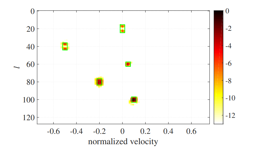
The final result of 1D-KST is shown in Figure 5. When looked together with Figure 3, it is clearly shown that all objects are well located in the grid cells at the midpoint time instant and their velocities are also measured with a high precision even for these so noisy OGMs22. Moreover, the occupies of every are well focused in the green box determined by 1D-KST's resolution, which is determined by (22) and the width of the spatial frequency window:
From this result, we can conclude that 1D-KST has a good performance for the point object in terms of OGM filtering and the extraction of motion information.
The results of the two dimensional test are shown in Figures 6 - 10. Similar to the one dimensional case, we choose the maximal feasible and minimal detectable speed to are set to evaluate the capability of 2D-KST in terms of velocity measurement. Different from one dimensional case, we use eight hypotheses of direction to match the possible moving directions in OGMs. Among all five moving objects, four are moving along the direction in the hypothesis sets, while the last one (#5) is moving near the middle direction between the hypothesis and the reverse direction of , but slightly close to . Through this setting, we can evaluate the performance when the true moving direction dose not match any hypotheses. To see the result more clearly, we decrease the map size in the two dimensional test. The detailed parameter setting used in this simulation can be seen in Table 1.
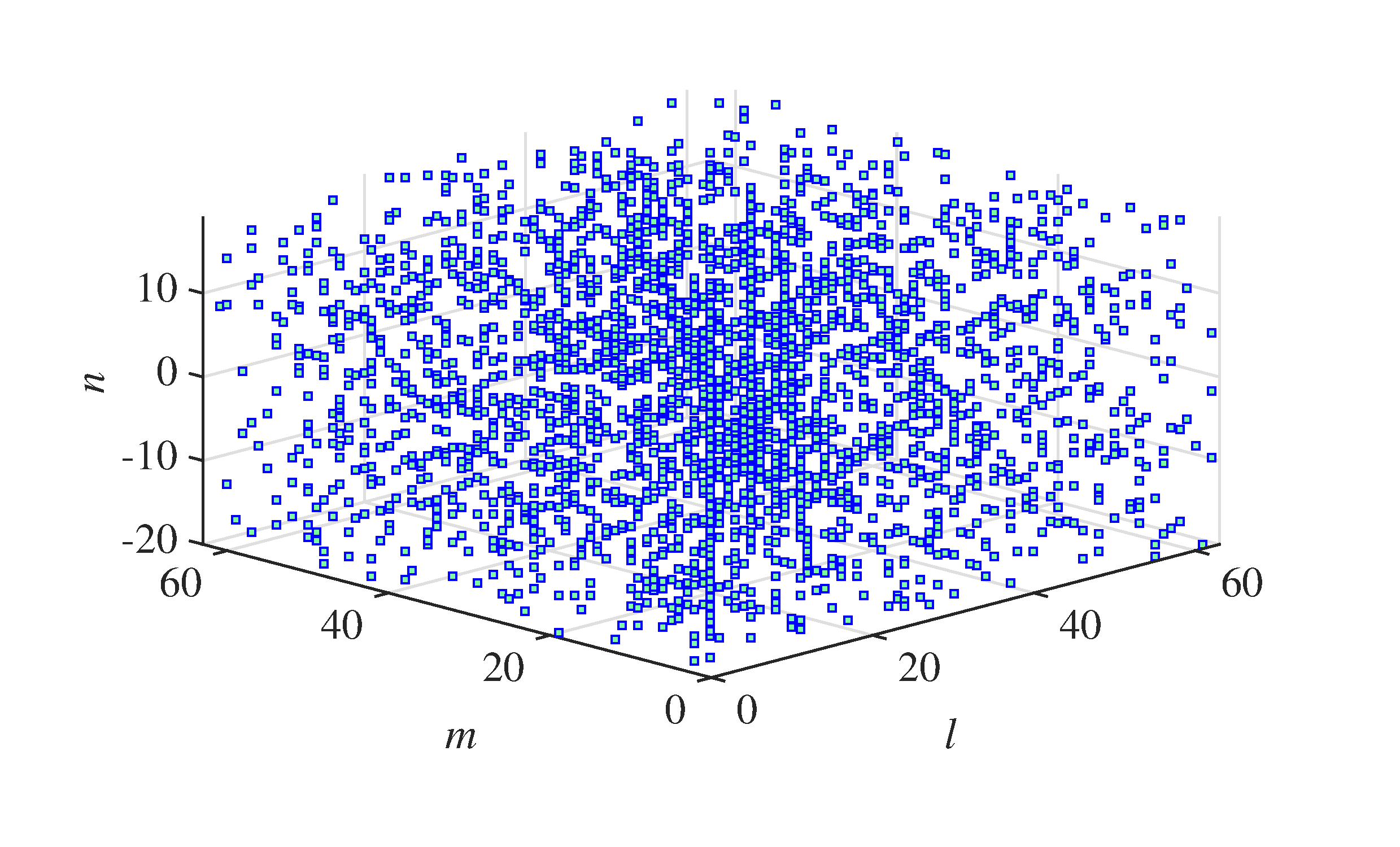
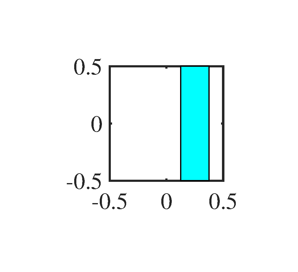
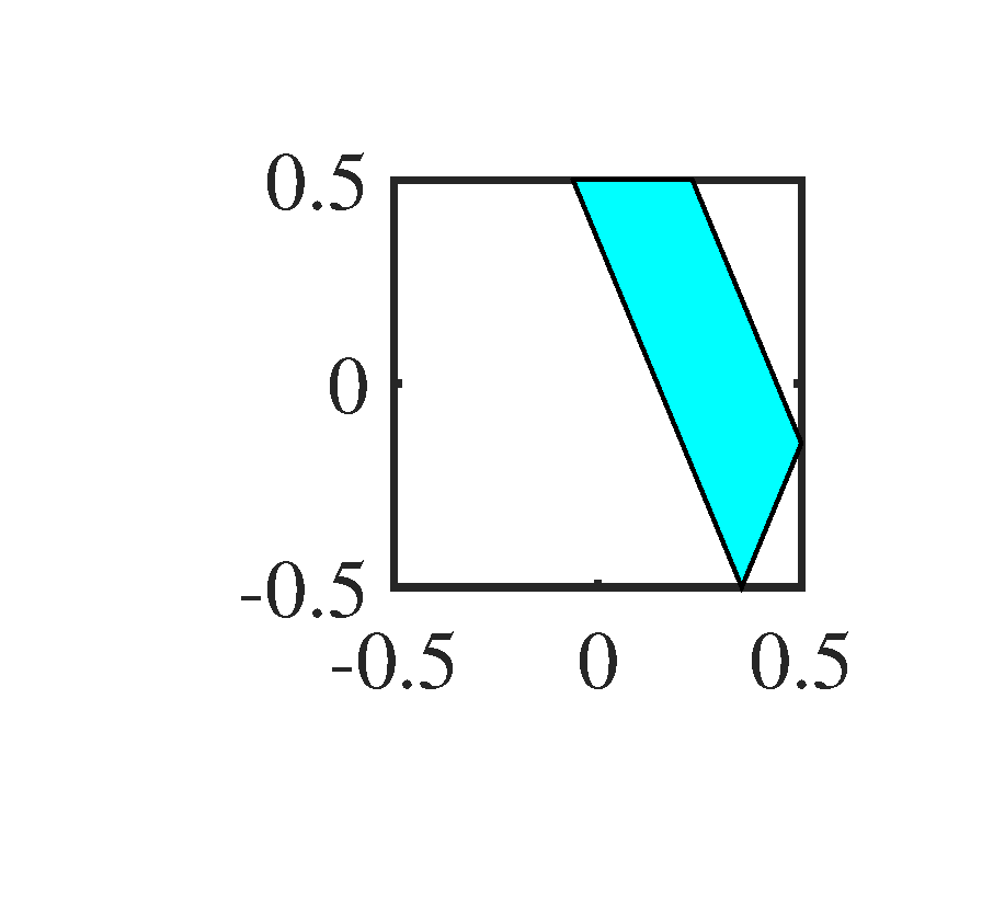
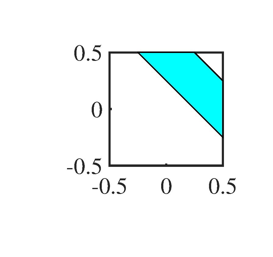
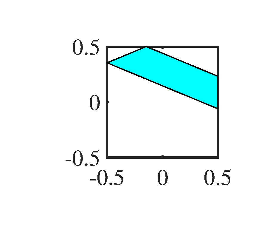
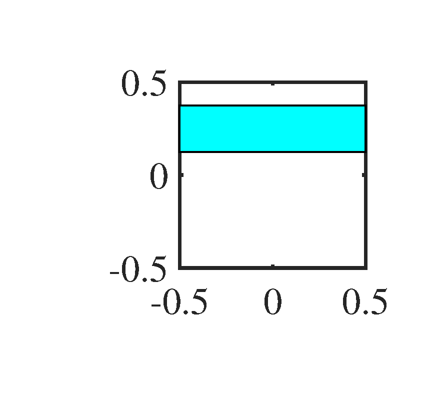
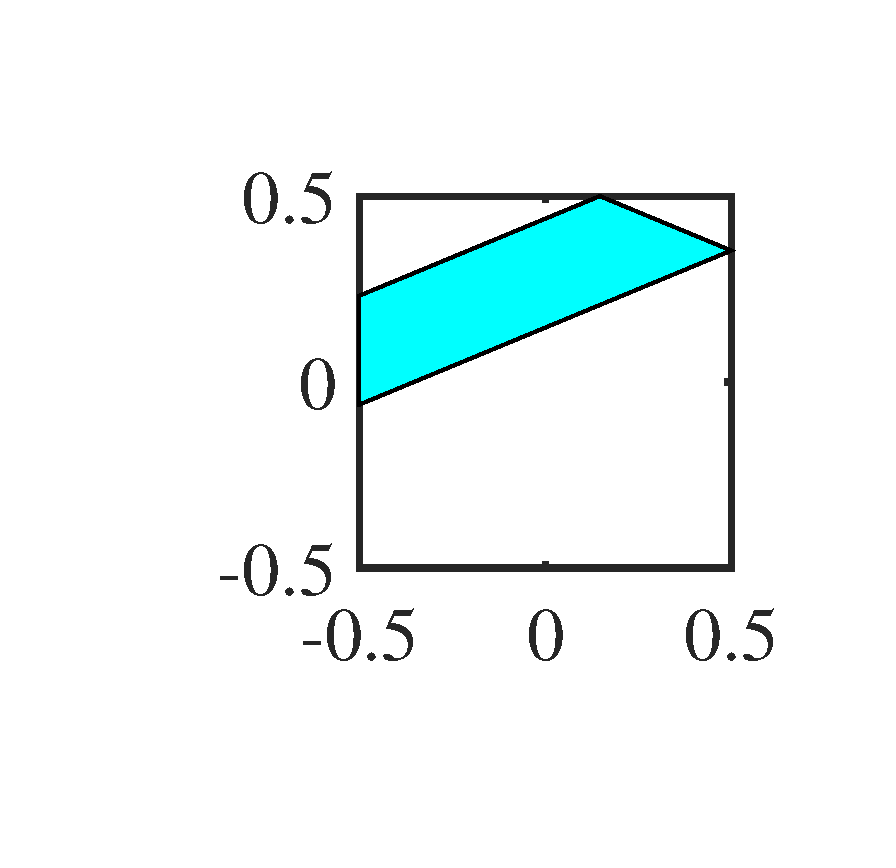
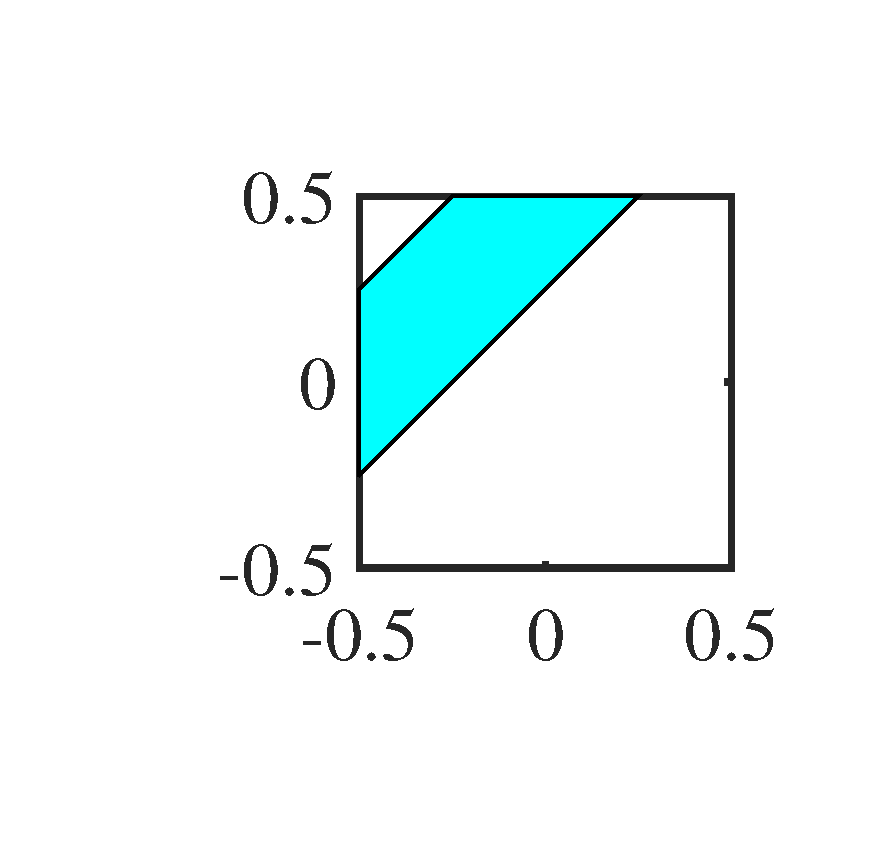
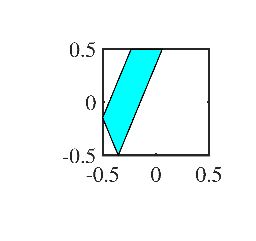
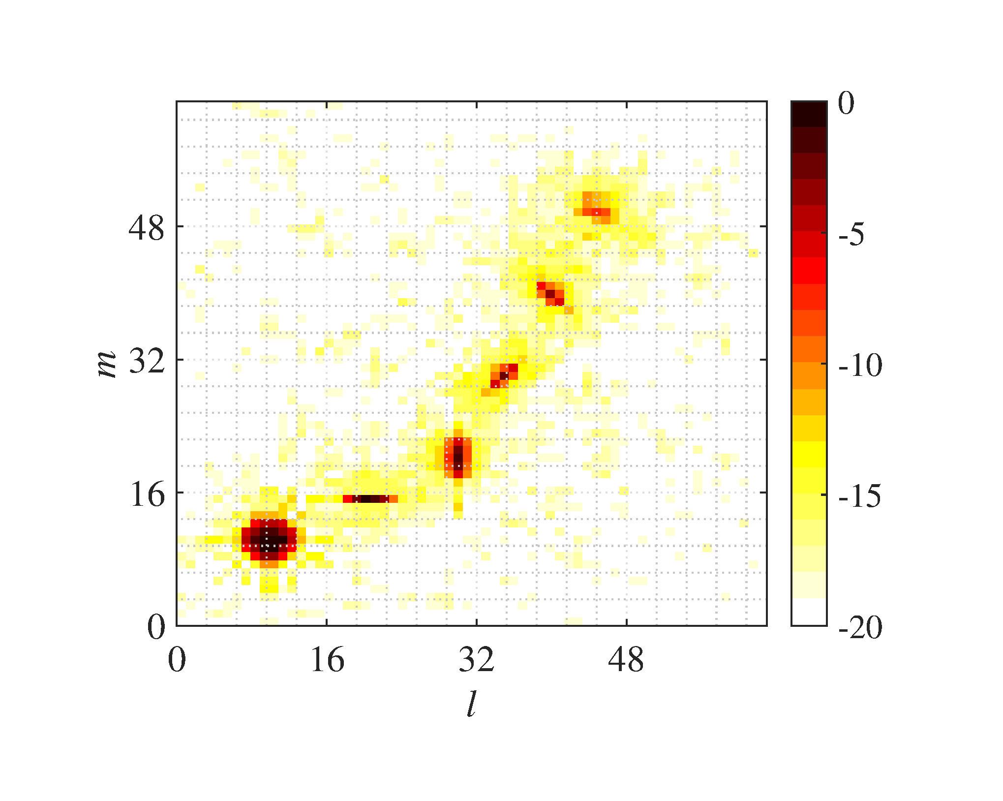
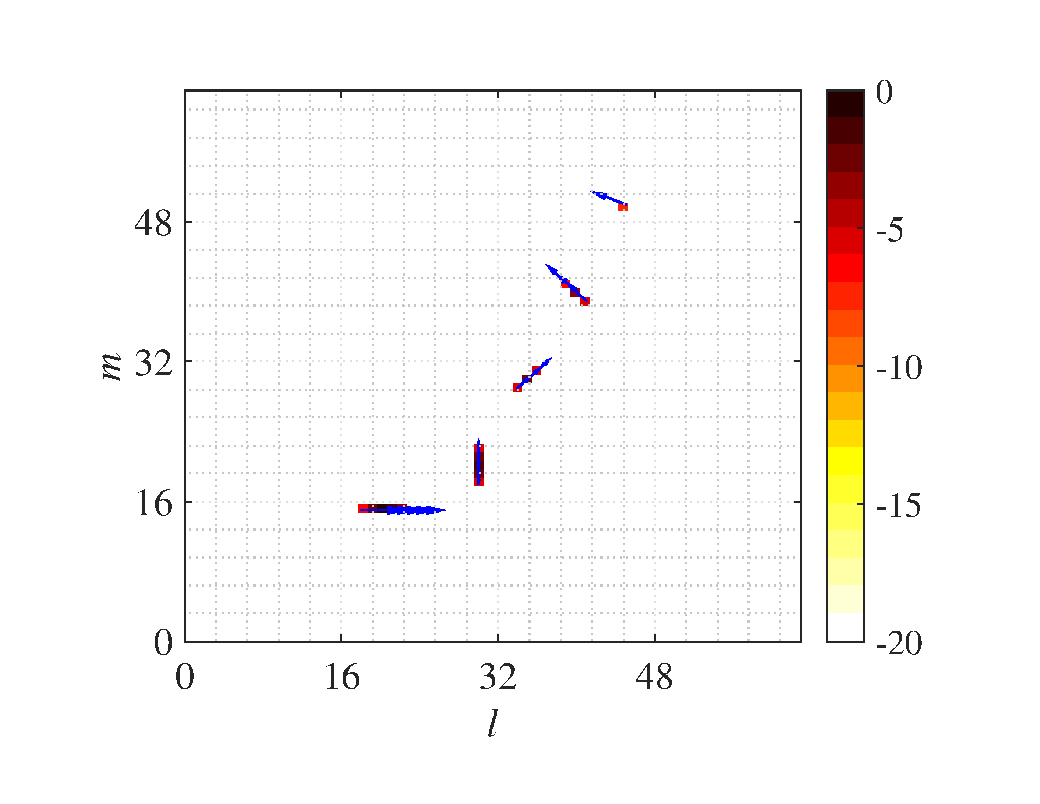
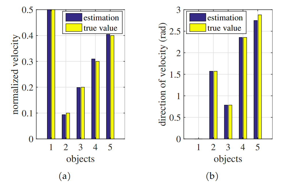
Figure 6 shows the noisy 2D-OGM sequence. It is very difficult to recognize the trajectory of each object by human eyes. To make the window more intuitive than the expression (1) to the reader, we show them in Figure 7. In principle, the counterpart of the spatial frequency window here is the directional filter in optical signal processing, this is also the reason why we call the second step of 2D-KST as directional filtering.
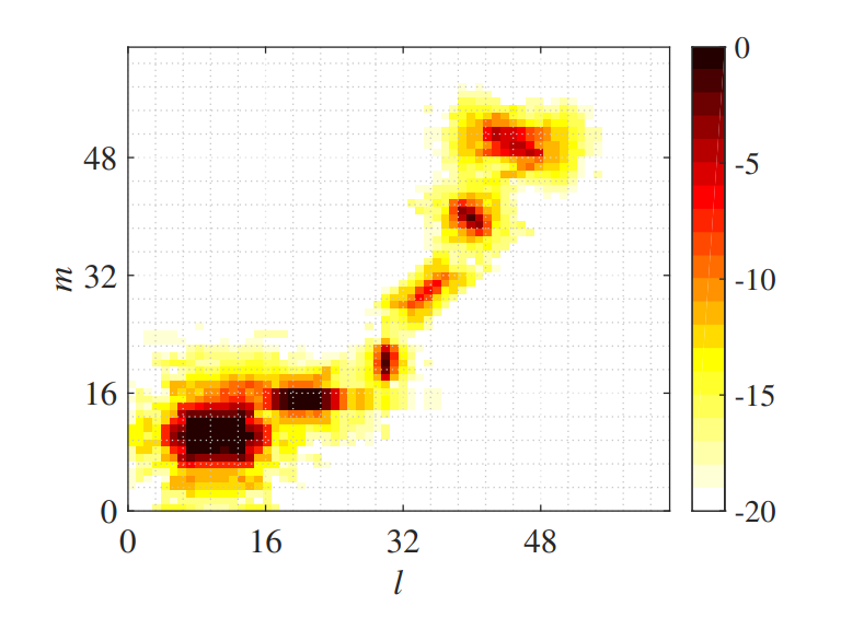
After the first merging step of MPD, the result of 2D-KST processing is shown in Figure 8, which can be regard as the filtered OGM at the time instant . Figure 8, we can found that the noise in the original OGM is almost filtered, and the grid cells in the vicinity of objects have a significant occupancy value. The occupancies in the yellow grid cells around each object are the leakage of occupancy in the corresponding object grid cell, which is the consequence caused by the window . Among all the six objects, the stationary object at behaves obviously isotropic, while the other moving objects behave the obvious directionality, which means that they have the biggest extent along their moving direction. Moreover, we can found that the grid cells near the mismatched one at have a relatively smaller value than those near the matched objects. Nonetheless, their values are at least twice as large as the values of those yellow grid cells. Thus, if we set the appropriate threshold , see (13), we can remove the leakage occupancies in the yellow cells but maintain those in the vicinity of the mismatched object grid cell. Furthermore, if our requirement is to extract the moving objects, we can filter the stationary one by setting the appropriate threshold , see (16).
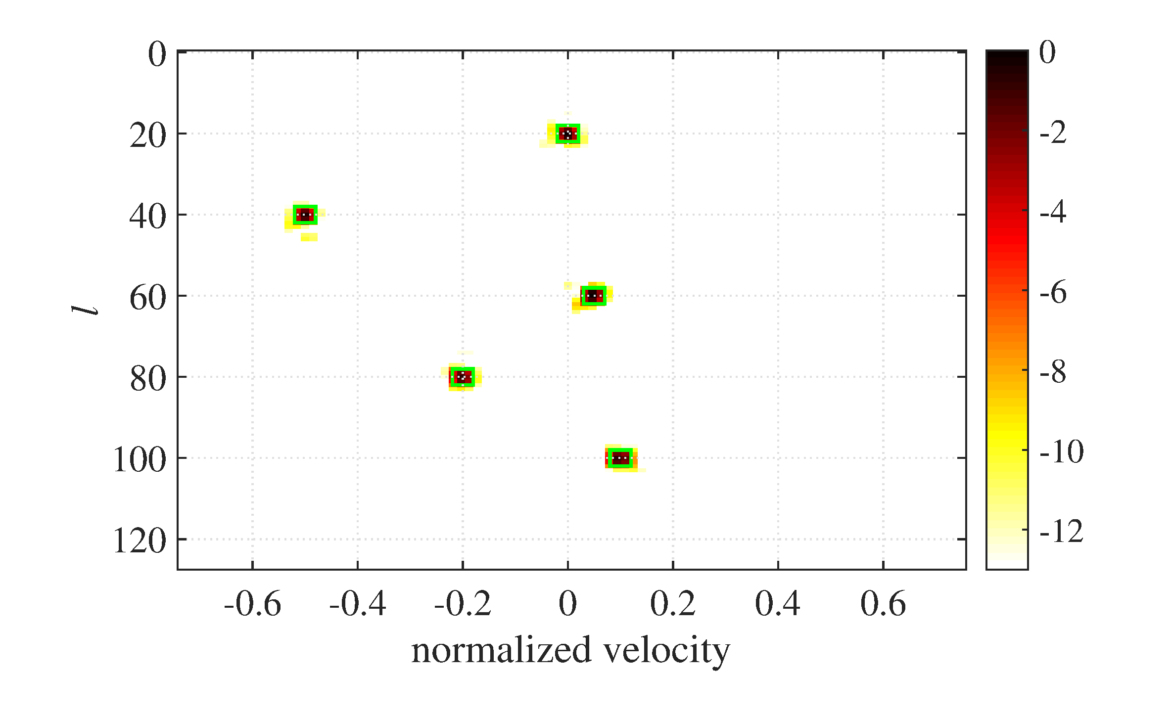
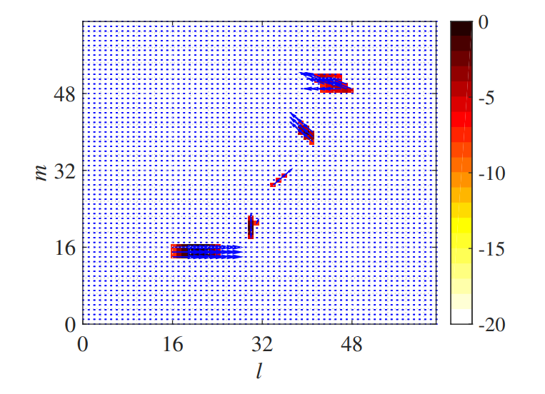
The result of 2D-KST after MPD processing is shown in Figure 9, where (-8dB) and are used, and where the blue arrows represent the velocity of the occupies in the corresponding cells, the length and pointing for the amplitude and the direction respectively. As can be seen from Figure 9, the stationary object has been removed successfully, although it has the maximal occupancy, while the five moving objects all persist in existing. What's more, the velocity measurements are highly in accordance with the ground truth in Table 1. To see it more obviously, the simple plot extractor is used, which extracts the local power maximum grid cells from the MPD results as the candidate detections and computes the occupancy weighted velocity as the velocity measurement of each candidate detection. The measurement results are shown in Figure 10, which suggest that 2D-KST has a good precision of velocity measurement for the point object and can be easily integrated with the plot extractor or other object clustering algorithm, such as FCTA [22].
The purpose of this experiment is to illustrate how the parameters of the spatial frequency window affect the output for different object sizes. Since the window parameters have the same effect on the output for the 1D and 2D cases and the 1D case is more easily to explain, we test two typical windows in one dimensional case for five different object sizes firstly. Through this test, some guidelines about how to choose the parameters for the spatial frequency window are derived. Then we validate these guidelines through 2D test for different object sizes. The size of each object used in this experiment is listed in Table 2, where the value means how many grid cells are occupied by this object. For 2D case, the two values correspond to the numbers of the occupied grid cells parallel and perpendicular to the direction of the velocity respectively. The other parameters are the same as Table 1 if without any special explanations.
| object label | #0 | #1 | #2 | #3 | #4 | #5 |
|---|---|---|---|---|---|---|
| 1D case | 5 | 4 | 1 | 3 | 2 | – |
| 2D case | 6,3 | 3,3 | 1,1 | 2,1 | 2,2 | 3,2 |
The responses to the two typical windows in one dimensional case to the five object sizes are shown in Figure 11.
As can be seen from Figure 1111(a) and 11(b), the wide window has a better resolution whether for the position or for the velocity, because it has a wider window and a higher reference spatial frequency . See (2) and (22) for the formulas about the KST resolution. But the large objects, object #0 at cell 20 and object #1 at cell 40 are split into two parts because the bandpass spatial filter is used in our KST approach. However, the two parts, the head and the tail, are both in the extent of the corresponding object which is represented by the green box. Fortunately, this split outcome may be accepted for many applications, such as CTM building [12] or DATMO using FCTA [22].
If it can not be accepted, the narrow window can be used instead. As shown in Figure 1111(b), all objects are focused in the corresponding green box. However, the velocity resolution gets worsened as the lower used, and the object #2 at cell 60 has a negligible occupancy inside its green box since only very little proportion of its power can enter the narrow window.
In principle, we can get the following two empirical criteria for selecting the parameters of the spatial frequency:
, which ensures that the scaled time for each spatial frequency shown in Figure 1 has not too big gap with the one for . As a result, the average resolution of frequency for every cell can be approximated by the one of .
, where is the possible maximal size of the object along its moving direction. This criterion ensures that the object can be focused along their moving direction, because for the length continuous segment in OGM, its maximal effective spatial frequency is at . Only if this condition holds, the information of this object as a whole can be maintained.
In practice, we can choose the appropriate parameters of spatial frequency window to meet the above two criteria. But for those applications in which the moving objects have the significant difference in size, for example, the case of Figure 11, we can use multiple windows to match different object sizes, or use a uniform window but based on the multiple resolution grid cell maps for different sizes of objects. Along this path, it will result in a multiple resolution KST approach, which is beyond the scope of this paper and maybe the next step work in the future.
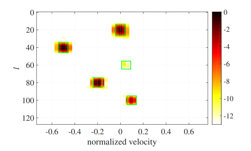
Next we validate the wide window in 2D case, the parameters can be seen in Table 1, through those objects in Table 2, where the extensions of all moving objects are no larger than 3 grid cells. The corresponding results are shown in Figure 12. From these results, we can conclude that when using the appropriate setting of spatial frequency window, the 2D-KST can perform very well for the extend objects when they have no too much difference in size.
Similar to the point object test, in order to demonstrate the potential capability of integrating with FCTA or other extend target tracking algorithms, we give the result of the plot extractor, which is shown in Table 3. As can be seen from Table 3, ten detections are achieved for those five moving objects altogether, and the average position is at the center of extend object, see Table 1 for the ground truth. Moreover, the velocity measurements also have a high precision, even for the mismatch one (#5), the maximal speed error is less than 0.05 and the direction of velocity is no more than 7 degrees among those three detections generated by this object.
| (deg) | object label | |||
| 1 | (20,14) | 0.5 | 0 | |
| 2 | (20,15) | 0.5 | 0 | #1 |
| 3 | (20,16) | 0.5 | 0 | |
| 4 | (30,20) | 0.09 | 87.1 | #2 |
| 5 | (34,29) | 0.20 | 45 | #3 |
| 6 | (36,31) | 0.20 | 45 | |
| 7 | (40,40) | 0.31 | 135 | #4 |
| 8 | (47,49) | 0.38 | 161.4 | |
| 9 | (45,50) | 0.35 | 171.6 | #5 |
| 10 | (43,51) | 0.38 | 161.4 |
Above all, as the point object test, it seems that 2D-KST has a good precision of velocity measurement for the extend object and can be easily integrated with the plot extractor or any other extend object tracking algorithm.
This paper developed a different way of extracting motion information from successive noisy OGMs based on a signal transformation by extending the KST in the radar signal processing community to the 1D and 2D spatial case. And the fast algorithm for the 2DS-KST is also given and has the proportional computational complexity with the 2D-FFT. Simulation results show that our method can extract the sub-pixel motions effectively from the sequence of very noisy OGMs, which has a wide use, in many application scenarios, such as the industrial field, airport and other indoor environment.
Further evaluation by real data, multi-resolution KST for complex scenarios, integration with Bayesian Occupancy Filter and CTMAP, and hypothesis merging method based on more complex velocity model, are worth being paid attentions in the next step.
 Copyright © 2024 by the Author(s). Published by Institute of Central Computation and Knowledge. This article is an open access article distributed under the terms and conditions of the Creative Commons Attribution (CC BY) license (https://creativecommons.org/licenses/by/4.0/), which permits use, sharing, adaptation, distribution and reproduction in any medium or format, as long as you give appropriate credit to the original author(s) and the source, provide a link to the Creative Commons licence, and indicate if changes were made.
 Chinese Journal of Information Fusion
ISSN: 2998-3371 (Online) | ISSN: 2998-3363 (Print)
Email: [email protected]

Portico
All published articles are preserved here permanently:
https://www.portico.org/publishers/icck/