

Chinese Journal of Information Fusion
ISSN: 2998-3371 (Online) | ISSN: 2998-3363 (Print)
Email: [email protected]

With the rapid development of remote sensing (RS) satellite technology, the quantity and quality of RS images have been significantly improved. Due to gradually realizing the significance of maritime rights and interests [1], a highly accurate and reliable RS ship images classification method is required.
The traditional RS ship images classification studies mainly focus on coarse-grained ship classification and most depend on shallow global features [2], which can only be used for simple classification task. In recent years, as the requirements for RS images classification becoming more detailed in military and civilian ocean resource utilization [3], fine-grained classification of RS ship images is becoming more and more significant. However, RS ship images can be confusing and difficult to distinguish, as the ships belonging to different category may appear very similar, and the content of RS images can be complex [4]. Fortunately, deep learning methods seem to be more effective and have made great achievement in computer vision field. In the task of fine-grained RS ship images classification, A push-and-pull network is proposed in [5], which integrated with the advances of contrastive learning to make the classification effective. Self-calibrated convolutions and class-balanced loss are introduced to the classification network by Chen et al. [6], to enrich features and overcome the class imbalance.
In addition to the powerful feature representation capability of the model, explainability is received the widespread attention in the last few years, which tries to make the decisions and mechanisms of the model more understandable to humans [7]. However, most of the existing fine-grained ship classification methods based on the end-to-end learning strategy provide infrequent interpretability, the models are only trained to match the datasets. If human could understand the region where models focus on or the mechanism how models make prediction in the task of fine-grained image classification, they may give more trust on the final predicted results. Visual attention mechanism has already been used in image classification to improve the performance of the model [8], and it also can yield heatmaps that indicate key regions for driving a model's decision. Notably, graph convolutional network (GCN) [9] becomes a hot network architecture, which could establish a graph structure by analyzing the relations between nodes [10]. Therefore, GCN could be used to capture and explore the intrinsic relationships of different regions in an image, contributing to improve the models' explainability. Some scholars have tried combining graph network with other networks to improve the performance or explainability of the model [11, 12, 13].
With the aforementioned consideration, we propose an explainable RS ship images classification framework based on graph network. In order to make people have a better understanding of the model's final prediction meanwhile not affecting the classification ability of the model, the local visual attention and graph network are combined in the proposed model to obtain the discriminative feature and explore the semantic relation of different parts of the target. As a result, the network can focus on the key regions of targets and then effectively learn the relations between them through graph structure. In contrast to alternative methodologies, our model could present the targets' parts it focused on and the relatively clear decision-making process without compromising the classification performance. The main contributions of this paper are as follows.
1) An explainable RS ship images classification network is proposed, to the best of our knowledge, we are the first to use the combination of convolutional neural network (CNN) and GCN in this field to explore the explainability of it.
2) By adding the local visual attention module (LVAM) to the feature extraction process, the network can pay attention to the key local regions which are used for final prediction. Moreover, attention maps may help users understand the decision-making progress from the human visual angle.
3) By introducing the GCN, it could help the proposed network capture the underlying association relationships between local regions that are important for the its final decision. The experimental results on two public ship classification datasets validate the classification ability and explainability of the proposed method.
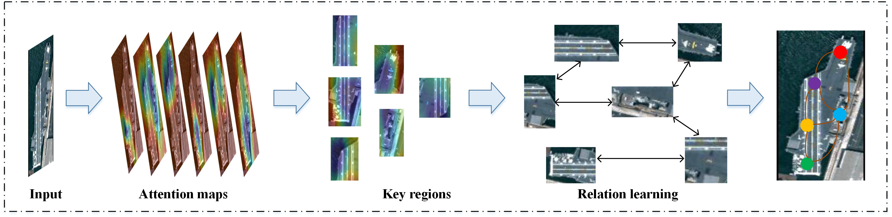
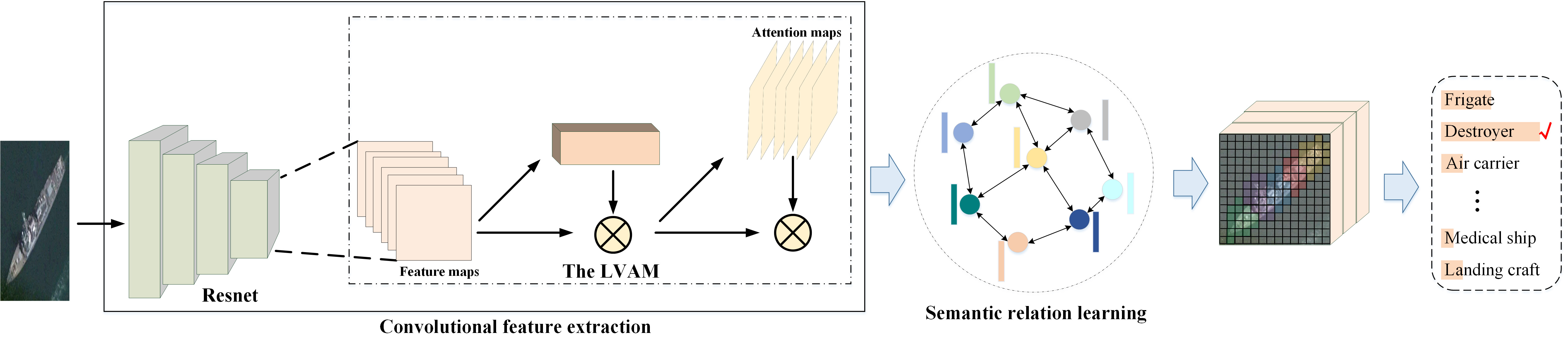
The overall framework proposed in this paper is shown in Figure 1, and there are mainly two parts, namely, convolutional feature extraction and semantic relation learning. The LVAM in feature extraction is to capture the important regions of the objects in input images, and then these local representations are further input to the relation learning part which utilizes GCN to exploit intrinsic relationships of the regions, providing more thorough explanations. Next, we will explain each of these components in detail.
Most existing deep neural network explanation methods only produce low-level attention maps, but they may not be intuitive for human to understand. The LVAM in the network is developed to capture key regions of the object and help improve model's explainability, and now we give a detailed introduction. As shown in Figure 1, when a RS ship image is input to the proposed network, the global high-level feature maps obtained from the last residual blocks of ResNet is represented as , where , , and represent the weight, height, and number of channels of feature maps, respectively. First, different sizes convolutional kernels are used to obtain the fused feature maps:
where denotes the size convolutional kernel, and represents the cat operation between feature maps in the channel dimension.
Then, the LVAM adopts a simple structure to obtain local attention maps , , where is the convolutional function with the kernel size of , and note that is the outputting channel number which indicates the number of key regions and is set in advance. Finally, the key regions of can be obtained according to the maximal value of the channel-wise position in . Furthermore, local attention loss function is designed to supervise this learning process, and we give detail introduction in Section 2.3.
Based on the local attention maps, we could get the visual explanations and be aware of the important object parts which are beneficial to the final decision. In this step, the GCN is further used to mine the semantic relations between them so as to make the obtained feature representation is more discriminative. The GCN utilizes node features and neighborhoods' relations to extract advanced features. A graph is defined as , where is the set consisting of nodes and represents the set of edges. Generally, the adjacency matrix is used to represent the edge relations between nodes. About a single-layer GCN, the process of graph convolution can be defined as:
where is the input feature matrix, is the output feature matrix, is the trainable matrix, and denotes the activation function.
As shown in Figure 2, in the proposed model, the regions obtained from the LVAM is regarded as the nodes to construct a graph. Specifically, according to the index of the maximal value in each local attention map, we average the fused features within each region as the graph nodes , which form the input feature matrix . So as to capture the regions' interrelationship, the adjacency matrix is defined as:
where means the Euclidean distance metric, which is used to measure the resemblance between graph nodes. After the GCN updating nodes' features according to equation (2), a convolution function with the kernel size of 1 1 is applied as the feature fusion module to obtain the discriminative features, and the convolution's output channel number is equal to the number of semantic classes in corresponding dataset. Then, the final feature representation vector is obtained through calculating the average of each feature map, so as to get the ship images' semantic labels rapidly and precisely.
The loss functions for training our model can be divided into two parts: local attention loss function and total loss function.
Generally, the attention maps may not focus on the discriminative parts of the objects. In order to make the model pay attention to different and important regions after the LVAM, the local attention loss function is designed to guide the attention learning process. Specifically, the definition is as follows:
where is the standard cross-entropy loss, indicates the prediction from output attention features of the LVAM, is the Pearson's correlation coefficient among different local attention features, and is the true label of the input, and are the hyper-parameters, which could balance the weight of corresponding part.
About the total loss function, we use cross-entropy loss function as the model's total classification loss, which provides a supervision signal over the feature learning process. It could be expressed as follows:
where indicates the model's final prediction, and is the true label of the input.
The final loss function for training is written as:
Two public datasets are adopted to verify the proposed model in subsequent experiments, and they are FGSC-23 [1] and FGSCR-42 [14]. The FGSC-23 dataset is a 23-category fine-grained RS ship classification dataset, and it contains totally 4080 ship images cropped from Google Earth public images and GF-1 satellite. The sizes of images range from 40 40 pixels to 800 800 pixels. The FGSCR-42 dataset is a lager fine-grained RS ship classification dataset, and it contains 42 categories and about 7776 RS images. The sizes of images range from 50 50 pixels to 1500 1500 pixels.
We conduct adequate experiments to demonstrate the effectiveness and explainability of our proposed model. In our experiments, the FGSC-23 dataset is divided into a training set and test set in a 8:2 ratio in accordance with [1], and we follow [14] to randomly select half of the images of each category from the dataset FGSCR-42 for training, while the rest for testing. Similarly, in order to get over the imbalanced sample problem, data augmentation operations are performed to supplement image samples of the fewer sample subclasses in the training set. The ResNet50 [15] pretrained on ImageNet is adopted to extract the high-level features from the input RS images in our network. All the models are trained for 80 epochs with a minibatch size of 16. The adaptive moment estimation (Adam) optimizer is employed for the training with an initial learning rate set at 5e-5.
| Dateset | Model | OA |
| FGSC-23 | Inception-v3 | 83.88 |
| DenseNet | 84.00 | |
| MobileNet | 84.24 | |
| Xception | 87.76 | |
| ME-CNN | 85.58 | |
| FDN | 82.30 | |
| B-CNN | 84.00 | |
| SIM | 86.30 | |
| P2Net | 87.27 | |
| ours | 88.85 | |
| FGSCR-42 | VGG19 | 77.36 |
| DenseNet | 88.69 | |
| ResNext-50 | 89.16 | |
| B-CNN | 89.53 | |
| RA-CNN | 91.63 | |
| DCL | 93.03 | |
| TASN | 93.51 | |
| SIM | 97.90 | |
| ours | 98.35 |
| Model | |||||||||||
| ResNet50 | 90.72 | 79.41 | 97.92 | 100.00 | 89.66 | 66.67 | 90.00 | 100.00 | 100.00 | 84.06 | 81.82 |
| ours | 87.63 | 94.12 | 93.75 | 100.00 | 96.55 | 64.44 | 85.00 | 100.00 | 100.00 | 81.16 | 87.88 |
| 40.00 | 85.19 | 66.67 | 100.00 | 100.00 | 81.82 | 88.14 | 66.67 | 81.36 | 83.33 | 96.77 | 88.89 |
| 70.00 | 94.44 | 72.22 | 100.00 | 90.91 | 77.27 | 94.92 | 94.44 | 86.44 | 100.00 | 100.00 | 83.33 |
| Model | ||||||||||
| ResNet50 | 95.27 | 100.00 | 77.14 | 100.00 | 97.47 | 96.02 | 100.00 | 91.67 | 96.77 | 79.14 |
| ours | 100.00 | 100.00 | 85.71 | 100.00 | 100.00 | 100.00 | 100.00 | 100.00 | 100.00 | 100.00 |
| 84.28 | 79.41 | 81.82 | 89.52 | 92.00 | 83.10 | 84.62 | 84.95 | 92.59 | 80.65 | 96.04 |
| 100.00 | 100.00 | 100.00 | 100.00 | 96.00 | 98.59 | 94.87 | 100.00 | 98.41 | 96.77 | 100.00 |
| Model | ||||||||||
| ResNet50 | 98.46 | 99.04 | 98.97 | 99.38 | 94.69 | 92.50 | 100.00 | 100.00 | 100.00 | 50.00 |
| ours | 100.00 | 100.00 | 99.74 | 99.38 | 100.00 | 100.00 | 100.00 | 100.00 | 91.67 | 50.00 |
| 100.00 | 0.00 | 85.29 | 100.00 | 80.00 | 100.00 | 33.33 | 88.89 | 0.00 | 76.57 | 65.52 |
| 100.00 | 50.00 | 100.00 | 100.00 | 100.00 | 100.00 | 66.67 | 88.89 | 33.33 | 94.39 | 91.38 |
The classification performance of the proposed method is evaluated by overall accuracy (OA), average accuracy (AA) and accuracy rate (AR) of each category. OA is the ratio of the correctly predicted images of total testing images, AA which seems more reasonable is the average of the accuracy of all categories, and AR is the ratio of correctly classified images among a category on the testing set.
To verify the performance of the proposed model, we compare the classification accuracy of the proposed method with other deep learning-based methods on two datasets aforementioned.
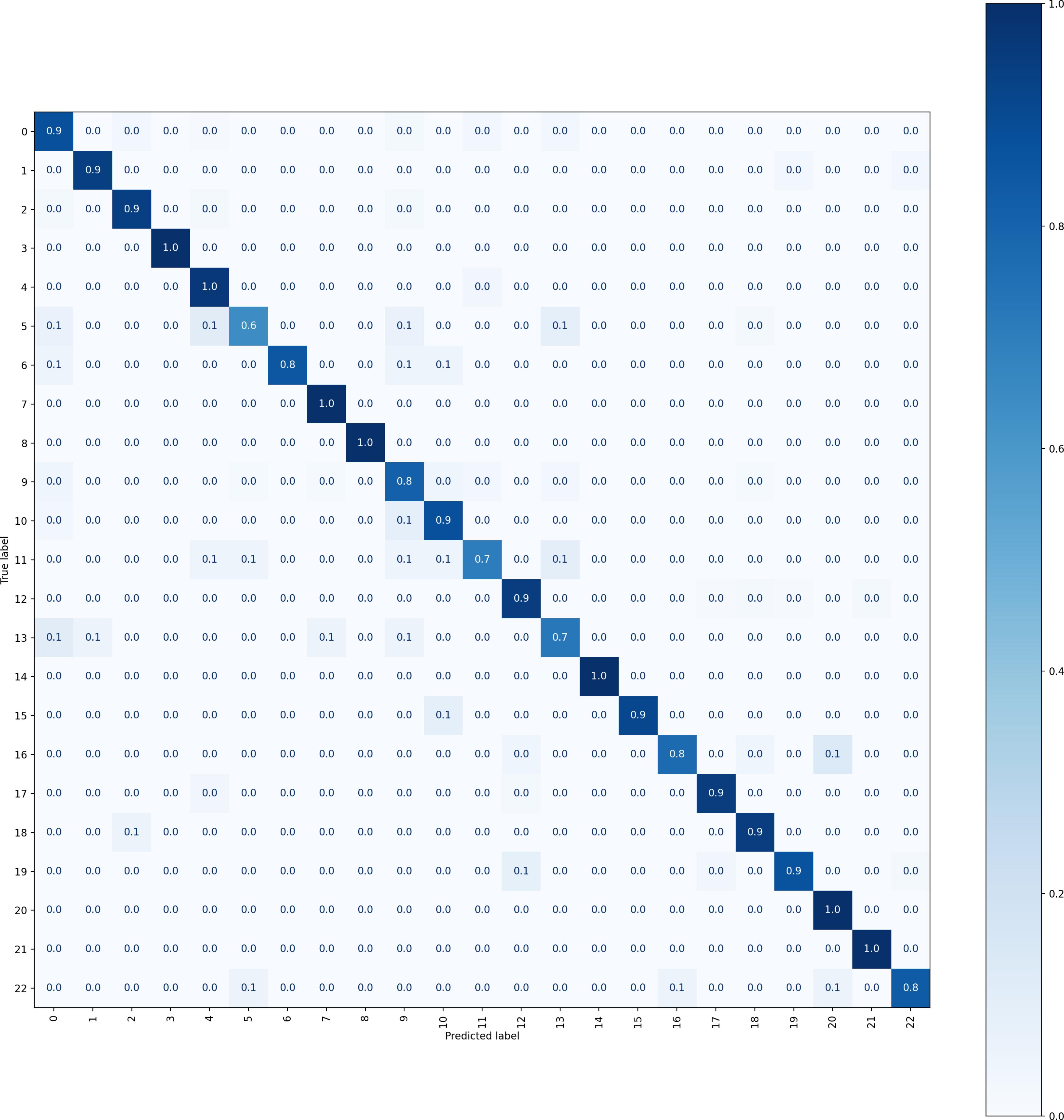
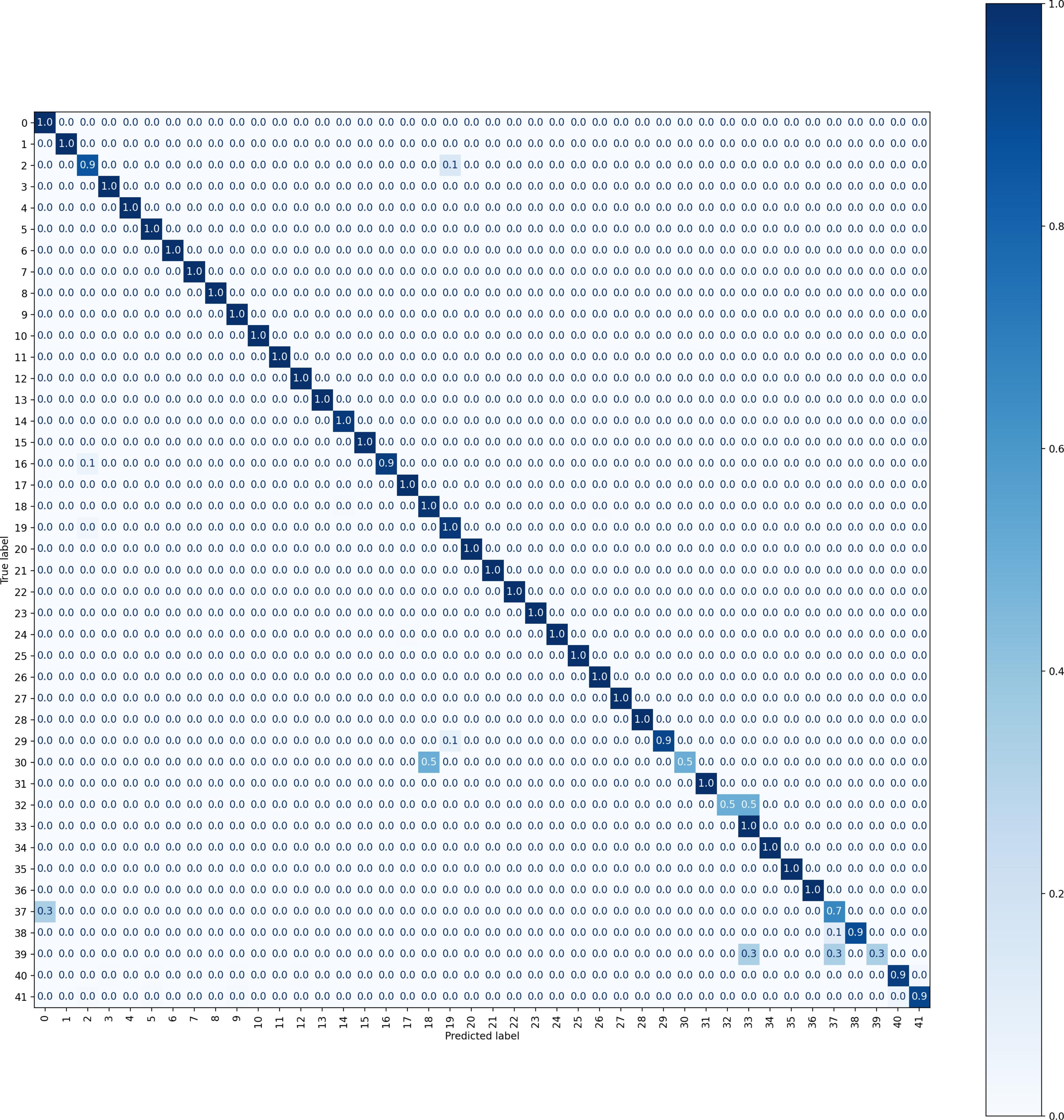
As shown in Table 1, we make comparison with various methods. Specifically, common CNN-based methods such as Inception-v3 [16], DenseNet [17], MobileNet [18], Xception [19], VGG19 [20], ResNext-50 [21] are included, in addition to B-CNN [22], RA-CNN [23], DCL [24], TASN [25], SIM [26] are fine-grained classification methods for natural images, and there are also some methods including FDN [27], ME-CNN [28], P2Net [5] which are proposed for the remote-sensing image classification. In Tables 2 and 3, we list the AR for each category of FGSC-23 and FGSCR-42 in the experiment respectively, and we compare the results of proposed method with the backbone network ResNet50. We can see that the performance of proposed method has achieved significantly enhanced compared with the representative common CNN models on both FGSC-23 and FGSCR-42 datasets and it also achieves superior results in contrast to other classification algorithms. This demonstrates the effectiveness of the model and shows the sufficiently good classification performance. In particular, the corresponding confusion matrixes of our method on FGSC-23 and FGSCR-42 datasets are displayed in Figures 3 and 4 respectively.
Ablation studies are conducted to evaluate the effectiveness of each part in the proposed model and analyze the influence on the experimental results. Specifically, we set up the ablation experiments about the modules of LVAM and GCN, and at the same time give the time spent on corresponding model testing on each dataset. As shown in the Table 4, R50 represents convolutional backbone Resnet50, we can see that the LVAM can help improve the learning performance notably compared with the same backbone network. This is because the LVAM focuses its attention on important parts of the ship images, which contribute to the final prediction. Furthermore, combined with GCN, the model's performance is further improved. This is mainly attributed to the semantic relationships between regions are exploited by the GCN, so that the model could learn more discriminative feature representation. Although the elapsed time for model testing has a certain degree of increase in the process of adding LVAM and GCN module, it is still very close to the convolutional backbone network. Besides, the proposed model has markedly enhanced the classification ability, which further demonstrates the effectiveness of our model.
| Dataset | Model | Test time | OA | AA | |
| FGSC-23 | R50 | 2.01 s | 85.21 | 85.18 | |
| R50LVAM | 2.09 s | 87.27 | 87.55 | ||
|
2.17 s | 88.85 | 89.33 | ||
| FGSCR-42 | R50 | 7.12 s | 89.83 | 84.41 | |
| R50LVAM | 7.17 s | 96.27 | 91.60 | ||
|
7.31 s | 98.35 | 93.71 |
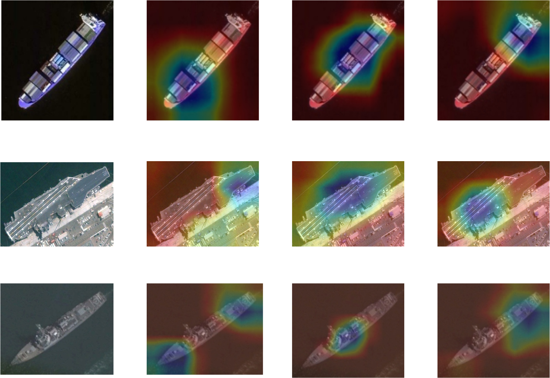
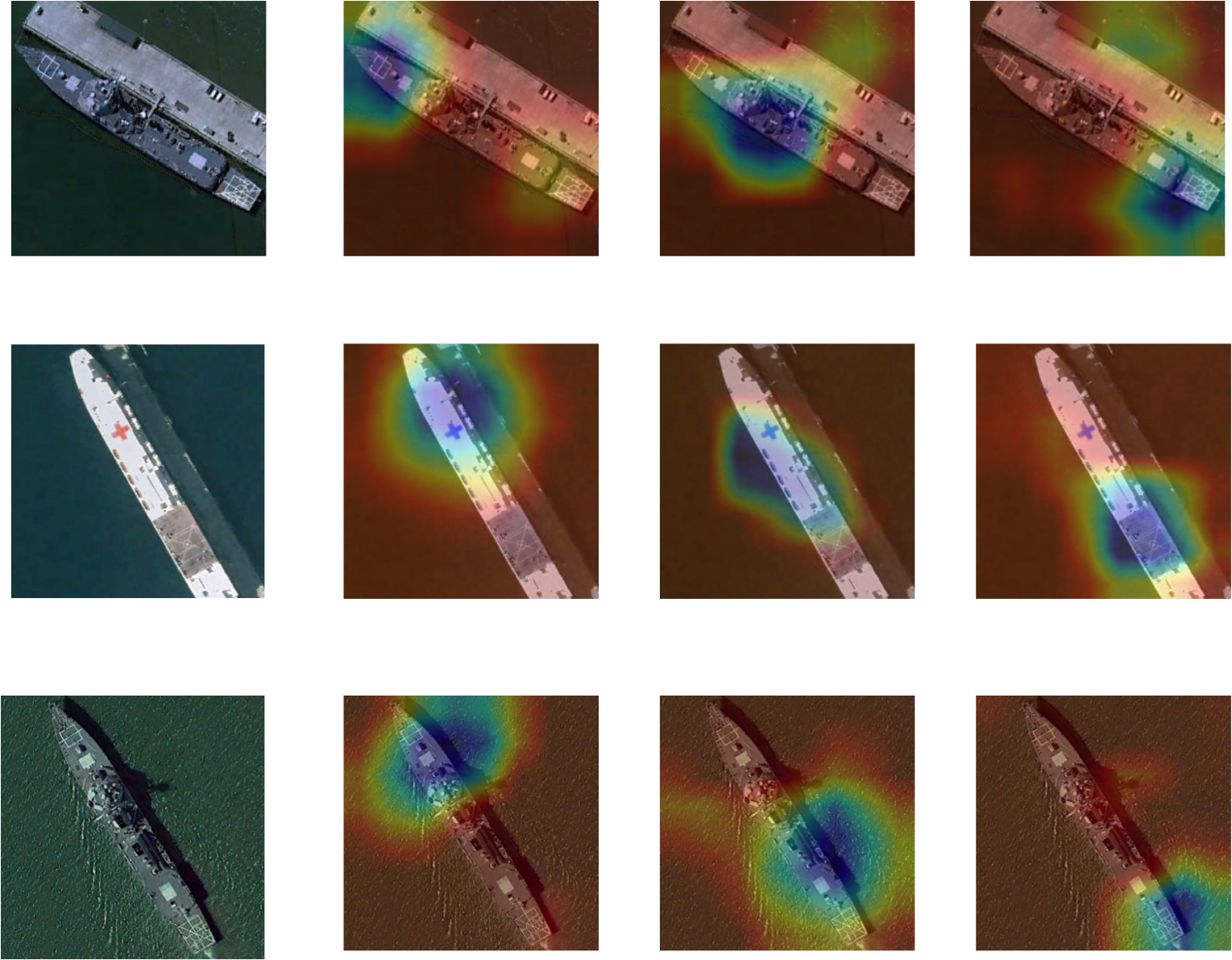
In this section, we simply select part representative attention maps as samples for analysis, and visualize them to verify the effectiveness of the designed LVAM, further to illustrate the effectiveness and explainability of the proposed method.
As shown in Figures 5 and 6, the first column displays input RS ship images, and different channel's attention maps are placed in the following last three columns. It can be seen that most areas of attention are focused on discriminative parts of the ship object and other irrelevant parts catch little attention in the image. Also, different channels concentrate on diverse local visual information of the objects. And the meaningful visualization information of provided by the model could make it easier for users to know key regions that the classification model pays attention to clearly, thus helping people better understand its decision-making progress. Meanwhile, the feature representation from LVAM will input to the graph network for further relation learning among the regions, which may contribute to enhancing the discriminative ability of the model. Combined the results in Table 4, we can conclude that the proposed method could provide explainable classification results and maintain an acceptable classification performance.
In this paper, an explainable classification method for RS ship images based on graph network is proposed. The method mainly consists of local visual attention and graph network two parts. When an image is input, the LVAM could make the model focus on important regions, and then the graph network is used to exploit the underlying relationships between them and get the final feature representation through the process of feature fusion. Extensive experiments and ablation studies on two public fine-grained ship classification datasets verify the effectiveness of the proposed model. Although we provide explainable attention maps visualization which may help people understand, we will seek a more powerful theory of explainable causal effect in future work.
 Copyright © 2024 by the Author(s). Published by Institute of Central Computation and Knowledge. This article is an open access article distributed under the terms and conditions of the Creative Commons Attribution (CC BY) license (https://creativecommons.org/licenses/by/4.0/), which permits use, sharing, adaptation, distribution and reproduction in any medium or format, as long as you give appropriate credit to the original author(s) and the source, provide a link to the Creative Commons licence, and indicate if changes were made.
 Chinese Journal of Information Fusion
ISSN: 2998-3371 (Online) | ISSN: 2998-3363 (Print)
Email: [email protected]

Portico
All published articles are preserved here permanently:
https://www.portico.org/publishers/icck/