Distributed Group Target Tracking under Limited Field-of-View Sensors Using Belief Propagation

Haiqi Liu; Xuqi Zhang; Bin Zhou; Bing Liu; Xiaojing Shen

doi:10.62762/CJIF.2025.314716

CiteScore

Impact Factor

Volume 2, Issue 3, Chinese Journal of Information Fusion

Volume 2, Issue 3, 2025

Submit Manuscript Edit a Special Issue

Table of Content

1. Introduction
2. Problem Formulation
3. Consensus-based DGTT Method
4. Algorithm Implementation
5. Experiments
6. Conclusion

Chinese Journal of Information Fusion, Volume 2, Issue 3, 2025: 194-211

Open Access | Research Article | 20 July 2025

Distributed Group Target Tracking under Limited Field-of-View Sensors Using Belief Propagation

Haiqi Liu 1

Xuqi Zhang 2 *

Bin Zhou 2

Bing Liu 1

Xiaojing Shen 1

1 School of Mathematics, Sichuan University, Chengdu, Sichuan 610064, China

2 Science and Technology on Electronic Information Control Laboratory, Chengdu 610036, China

* Corresponding Author: Xuqi Zhang, [email protected]

DOI: 10.62762/CJIF.2025.314716

Received: 02 April 2025, Accepted: 27 May 2025, Published: 20 July 2025

PDF (2.79 MB) Full-Text HTML XML

Article Metrics Cite This Article

Abstract

This paper considers the distributed group target tracking (DGTT) problem under sensors with limited and different field of views (FoVs). Usually, for the tracking of groups, targets within groups are closely spaced and move in a coordinated manner. These groups can split or merge, and the numbers of targets in groups may be large, which lead to more challenging issues related to data association, filtering and computational complexities. Particularly, these challenges may be further complicated in distributed fusion system architectures. To deal with these difficulties, we propose a consensus-based DGTT method within the belief propagation (BP) framework, which introduces undetected targets inside the FoV or new targets outside the FoV and performs the probabilistic track association via BP. Meanwhile, the obtained track association probabilities make it possible to exploit a probabilistic consensus fusion scheme for fusing local target densities. Furthermore, the proposed method exhibits computational scalability scaling only linearly on the numbers of group partitions, local measurements and neighboring sensors, and scaling quadratically on the number of targets. Numerical results validate the performance of the proposed method.

Keywords

group target tracking

distributed sensor network

consensus fusion

scalability

belief propagation

1. Introduction

Recently, the group target tracking (GTT) problem has become increasingly important and drawn great attention, which is an integral part of many applications in different fields, including battlefield surveillance [1], traffic control [2], robotics [3], ecology [4], etc. When compared to multi-target tracking groups not only suffers the difficulties such as missed detections, clutter, measurement origin uncertainty [5, 6], but also encounters the group structure uncertainty caused by group merging or splitting [7], which result in more complex issues related to data association, filtering, and computation.

Benefiting from the rapid development in communication and sensing technologies, the sensor network consisting of multiple interconnected sensors with sensing, communication and processing capabilities provides a desirable platform for the challenging target tracking applications, since the network system provides more information in time and space and makes it possible to overcome the lack of target observability from individual sensors with limited FoVs. In particular, distributed sensor network (DSN) has aroused tremendous interest as a result of its attractive merits such as scalability, flexibility, and robustness to faulty sensors. The optimal fusion rule is given in [8], while the computational difficulty of the common information among sensors limits its use, promoting the development of robust suboptimal fusion rules. Consensus provides a powerful tool for the distributed computation over networks, which aims to achieve the global fusion over the DSN by iterating local fusion steps among neighboring sensors. From a probability density perspective, consensus-based distributed fusion is actually an iterative calculation of the local Kullback-Leibler average (KLA) of the state probability density functions (pdfs) among neighboring sensors [9]. The KLA fusion rule [9] is also known as the generalized covariance intersection (GCI) [10, 11] or the exponential mixture density (EMD) [12, 13], belonging to the type of geometric average fusion of local pdfs. Furthermore, some studies focus on another type of arithmetic average fusion can refer to [14, 15]. Regarding the two fusion types, geometric average fusion is more sensitive to missed detections, whereas arithmetic average fusion is more sensitive to clutter [16]. Based on the robust fusion rule, a variety of distributed MTT methods have been investigated, e.g., probability hypothesis density (PHD) with EMD [13], cardinalized PHD with KLA [17], Labeled multi-Bernoulli with GCI [18], etc. Most of the aforementioned studies are presented without FoV limitations, while the conventional KLA fusion rule performs poorly when sensors in the network have limited and different FoVs [19]. To overcome this issue, some improvement methods are proposed [20, 21].

Recently, a powerful BP method has attracted substantial attention in the target tracking community[22]. The BP method can efficiently compute the approximations of the marginal posterior pdfs or probability mass functions (pmfs) for the random variables of interest, providing a scalable solution to the challenging probabilistic data association problem in MTT [23]. Based on the BP scheme, various scalable target tracking algorithms have been proposed for MTT from different perspectives, e.g., scalable MTT methods for tracking unknown number of targets [24, 23], maneuvering MTT [25, 26], simultaneous cooperative self-localization and MTT [27], etc. Recently, a variant of the LMB-GCI method for DMTT, which does not have FoV limitations, has been proposed by integrating BP to address soft (i.e., probabilistic) label association [28]. This approach demonstrates better performance compared to those using a hard label association scheme. Additionally, other BP-based algorithms for extended target tracking can be found in [29] and [30]. In the context of GTT, a group expectation maximization BP method has been proposed for tracking coordinated group targets [31]. To deal with group targets and ungrouped targets seamlessly, a scalable group target belief propagation (GTBP) method is proposed [32]. Given its strengths in estimation accuracy, computational complexity, and implementation flexibility [24], BP could prove to be a highly effective tool for addressing the challenges in DGTT.

In this paper, we consider the DGTT problem under sensors with limited and different FoVs, and our main contributions are outlined below:

We present a consensus-based distributed GTBP algorithm (DGTBP) for DSN. To address the target identity inconsistency among local sensors due to varying FoVs, we incorporate the undetected targets inside the FoV and new targets outside the FoV for track association. We then efficiently compute the marginal track association probabilities using BP, which are utilized for the consensus fusion in a probabilistic manner.
We clarify the computational complexity and scalability of DGTBP. It exhibits computational scalability that scales linearly in the numbers of group partitions, local measurements and neighboring sensors, while scaling quadratically in the number of targets. Numerical results verify the effectiveness and scalability of DGTBP.

The remainder of this paper is outlined as follows. Section 2 introduces the problem background and methodology. Section 3 presents the proposed consensus-based DGTT method, followed by a particle-based algorithm implementation given in Section 4. The numerical experiments and comparison results are shown in Section 5. To the end, we conclude this paper in Section 6.

2. Problem Formulation

2.1 Description of DSN

This paper considers the GTT problem in a DSN, where the sensors have limited and different FoVs. Generally, there is no fusion center in the DSN, and each sensor is restricted to processing local data and exchanging information with its neighboring sensors. For ease of representation, the DSN is described by a directed graph $\mathcal{D}:=(\mathcal{S},\mathcal{E})$ , where $\mathcal{S}:=\{1,\ldots,S\}$ and $\mathcal{E}\subseteq\mathcal{S}\times\mathcal{S}$ are the set of nodes and the set of edges between nodes, representing sensors and sensor connections, respectively. Here, $(s,s^{\prime})\in\mathcal{E}$ if and only if sensor $s$ can receive information from sensor $s^{\prime}$ . For each sensor $s\in\mathcal{S}$ , we denote $\mathcal{C}_{s}:=\{s^{\prime}\in\mathcal{S}:(s,s^{\prime})\in\mathcal{E}\}$ as the set of its neighboring sensors, i.e., these sensors in the network that may transmit information to sensor $s$ . According to the definition, $(s,s)$ belongs to $\mathcal{E}$ for any $s\in\mathcal{S}$ , and thus $s\in\mathcal{C}_{s}$ for any $s\in\mathcal{S}$ . The FoV of sensor $s$ is denoted by $FOV_{s}$ .

2.2 Consensus on the Kullback–Leibler Average

Consensus algorithms provide a powerful tool for distributed averaging, which aim to reach a consensus over the DSN by iteratively performing the local fusion of each sensor among its neighboring sensors. Suppose that at each sensor $s$ of the DSN, a pdf $p_{s}(\mathbf{x})$ representing the local information is available, where $\mathbf{x}$ is a random vector of interest. The weighted KLA pdf $p(\mathbf{x})$ among these local pdfs $p_{s}(\mathbf{x})$ is defined by [9]:

\displaystyle p:=\arg\min_{p}\sum_{s\in\mathcal{S}}\pi_{s}D_{KL}(p\ \|\ p_{s})

where the weights $\pi_{s}$ satisfying $\sum_{s\in\mathcal{S}}\pi_{s}=1$ and $\pi_{s}\geq 0$ , and $D_{KL}(p\ \|\ p_{s})$ is the Kullback-Leibler Divergence between the pdfs $p(\mathbf{x})$ and $p_{s}(\mathbf{x})$ ,

\displaystyle D_{KL}(p\ \|\ p_{s}):=\int p(\mathbf{x})\log\frac{p(\mathbf{x})}% {p_{s}(\mathbf{x})}\mathrm{d}{\mathbf{x}}

Further, the KLA pdf $p(\mathbf{x})$ defined in (1) is given by

\displaystyle p(\mathbf{x})=\frac{\prod\limits_{s\in\mathcal{S}}\big{(}p_{s}(% \mathbf{x})\big{)}^{\pi_{s}}}{\int\prod\limits_{s\in\mathcal{S}}\big{(}p_{s}(% \mathbf{x})\big{)}^{\pi_{s}}\mathrm{d}{\mathbf{x}}}

which requires all local pdfs $p_{s}(\mathbf{x}),s\in\mathcal{S}$ . From a distributed way, the following consensus iteration updates the local average of each sensor by fusing the local information of its own and the received information from its neighboring sensors.

\displaystyle p_{s}^{\left[\ell+1\right]}(\mathbf{x})=\frac{\prod\limits_{s^{% \prime}\in\mathcal{C}_{s}}\big{(}p_{s^{\prime}}^{\left[\ell\right]}(\mathbf{x}% )\big{)}^{\pi_{s,s^{\prime}}}}{\int\prod\limits_{s^{\prime}\in\mathcal{C}_{s}}% \big{(}p_{s^{\prime}}^{\left[\ell\right]}(\mathbf{x})\big{)}^{\pi_{s,s^{\prime% }}}\mathrm{d}{\mathbf{x}}}

where $\pi_{s,s^{\prime}}$ are suitable non-negative weights satisfying $\sum_{s^{\prime}\in\mathcal{C}_{s}}\pi_{s,s^{\prime}}=1$ for $s\in\mathcal{S}$ , $\ell$ denotes the number of iterations, and the iteration is initialized by setting $p_{s}^{\left[0\right]}(\mathbf{x})=p_{s}(\mathbf{x})$ .

2.3 System Model

At time $k$ , each potential target (PT) of a local sensor $s$ is either a legacy PT (i.e., a PT survived from time $k-1$ to time $k$ ) or a new PT (i.e., a newly detected target at time $k$ ). That is, the PTs can be divided into two categories at each time step, namely the legacy PTs and the new PTs. Let $\underline{\mathbf{x}}_{k,s}^{(i)}$ be the state vector of the legacy PT $i$ at time $k$ , consisting of the target position and possibly further parameters (e.g., velocity and acceleration), where $i\in\{1,\ldots,n_{k,s}\}$ and $n_{k,s}$ is the number of the legacy PTs at time $k$ . The detections of the legacy PTs are modeled by the binary existence variables $\underline{r}_{k,s}^{(i)}\in\{0,1\}$ , i.e., $\underline{\mathbf{x}}_{k,s}^{(i)}$ exists at time $k$ if and only if $\underline{r}_{k,s}^{(i)}=1$ . We denote $\underline{\mathbf{x}}_{k,s}:=[\underline{\mathbf{x}}_{k,s}^{(1)\mathrm{T}},% \ldots,\underline{\mathbf{x}}_{k,s}^{(n_{k,s})\mathrm{T}}]^{\mathrm{T}}$ and $\underline{\mathbf{r}}_{k,s}:=[\underline{r}_{k,s}^{(1)},\ldots,\underline{r}_% {k,s}^{(n_{k,s})}]^{\mathrm{T}}$ as the joint state vector and existence vector of the legacy PTs at time $k$ , respectively. Let $1_{FOV_{s}}(\cdot)$ denotes the indicator function that $1_{FOV_{s}}(\underline{\mathbf{x}}_{k,s}^{(i)})=1$ if $\underline{\mathbf{x}}_{k,s}^{(i)}$ is inside the FoV of sensor $s$ and otherwise $1_{FOV_{s}}(\underline{\mathbf{x}}_{k,s}^{(i)})=0$ .

Assume that at time $k$ , sensor $s$ receives $m_{k,s}$ measurements and the joint measurement vector is denoted as $\mathbf{z}_{k,s}:=[\mathbf{z}_{k,s}^{(1)\mathrm{T}},\ldots,\mathbf{z}_{k,s}^{(% m_{k,s})\mathrm{T}}]^{\mathrm{T}}$ . To incorporate the newly detected targets at time $k$ , $m_{k,s}$ new PT states $\overline{\mathbf{x}}_{k,s}^{(m)}$ , $m=1,\ldots,m_{k,s}$ are introduced, where each $\overline{\mathbf{x}}_{k,s}^{(m)}$ corresponds to the measurement $\mathbf{z}_{k,s}^{(m)}$ . The detections of the new PTs are also modeled by the binary existence variables $\overline{r}_{k,s}^{(m)}\in\{0,1\}$ , i.e., a measurement $\mathbf{z}_{k,s}^{(m)}$ is generated by a new PT $\overline{\mathbf{x}}_{k,s}^{(m)}$ if and only if $\overline{r}_{k,s}^{(m)}=1$ . We denote $\overline{\mathbf{x}}_{k,s}:=[\overline{\mathbf{x}}_{k,s}^{(1)\mathrm{T}},% \ldots,\overline{\mathbf{x}}_{k,s}^{(m_{k,s})\mathrm{T}}]^{\mathrm{T}}$ and $\overline{\mathbf{r}}_{k,s}:=[\overline{r}_{k,s}^{(1)},\ldots,\overline{r}_{k,% s}^{(m_{k,s})}]^{\mathrm{T}}$ as the joint state vector and existence vector of the new PTs, respectively. Notably, the new PTs at time $k$ become the legacy PTs when receiving new measurements at time $k+1$ , which means that the number of the legacy PTs at time $k+1$ is updated by $n_{k+1,s}=n_{k,s}+m_{k,s}.$ Since the number of PTs would increase with the accumulation of sensor measurements, we consider at most $N_{s}$ PTs at any time for sensor $s\in\mathcal{S}$ and perform a pruning step at each time step to remove unlikely PTs.

In GTT, the group structure describes the connection between targets, which is a premise of the modeling of the evolution of targets. In this paper, we make the convention that at any time $k$ , only the group structure of the confirmed legacy PTs (that have been declared to exist at the current time) is considered, and each confirmed legacy PT can be partitioned to only one group in a possible group structure. Concretely, we use a group partition vector $\underline{\mathbf{g}}_{k,s}:=[\underline{g}_{k,s}^{(1)},\ldots,\underline{g}_% {k,s}^{(n_{k,s})}]^{\mathrm{T}}$ to denote the group structure of all legacy PTs at time $k$ , where the element $\underline{g}_{k,s}^{(i)}>0$ if $\underline{\mathbf{x}}_{k,s}^{(i)}$ is confirmed and $\underline{g}_{k,s}^{(i)}=0$ otherwise. Furthermore, the group structure of the new PTs at time $k$ is denoted by the vector $\overline{\mathbf{g}}_{k,s}$ with zero entries, and we denote the number of groups partitioned by $\underline{\mathbf{g}}_{k,s}$ as $n(\underline{\mathbf{g}}_{k,s}):=\max\{\underline{g}_{k,s}^{(1)},\ldots,% \underline{g}_{k,s}^{(n_{k,s})}\}$ .

The unknown association between legacy PTs and measurements at time $k$ can be described by a target-oriented association vector $\mathbf{a}_{k,s}:=[a_{k,s}^{(1)},\ldots,a_{k,s}^{(n_{k,s})}]^{\mathrm{T}}$ , where the element $a_{k,s}^{(i)}=m$ if the PT $\underline{\mathbf{x}}_{k,s}^{(i)}$ generates the measurement $\mathbf{z}_{k,s}^{(m)},m\in\left\{1,\ldots,m_{k,s}\right\}$ at time $k$ and $a_{k,s}^{(i)}=0$ otherwise. Following [22, 24, 23], we also use a measurement-oriented association vector $\mathbf{b}_{k,s}:=[b_{k,s}^{(1)},\ldots,b_{k,s}^{(m_{k,s})}]^{\mathrm{T}}$ , where the element $b_{k,s}^{(m)}=i$ if the measurement $\mathbf{z}_{k,s}^{(m)}$ originates from the PT $\underline{\mathbf{x}}_{k,s}^{(i)},i\in\left\{1,\ldots,n_{k,s}\right\}$ and $b_{k,s}^{(m)}=0$ otherwise. The expression of $\mathbf{b}_{k,s}$ is redundant with $\mathbf{a}_{k,s}$ , that is, one of the two association vectors is determined and the other is determined as well.

We denote the joint vectors of all the PT state, the existence variable and the group partition at time $k$ as $\mathbf{x}_{k,s}:=[\underline{\mathbf{x}}_{k,s}^{\mathrm{T}},\overline{\mathbf% {x}}_{k,s}^{\mathrm{T}}]^{\mathrm{T}}$ , $\mathbf{r}_{k,s}:=[\underline{\mathbf{r}}_{k,s}^{\mathrm{T}},\overline{\mathbf% {r}}_{k,s}^{\mathrm{T}}]^{\mathrm{T}}$ and $\mathbf{g}_{k,s}:=[\underline{\mathbf{g}}_{k,s}^{\mathrm{T}},\overline{\mathbf% {g}}_{k,s}^{\mathrm{T}}]^{\mathrm{T}}$ , respectively. Let $\mathcal{R}_{k,s}$ , $\underline{\mathcal{R}}_{k,s}$ and $\underline{\mathcal{G}}_{k,s}$ be the sets of all possible $\mathbf{r}_{k,s}$ , $\underline{\mathbf{r}}_{k,s}$ and $\underline{\mathbf{g}}_{k,s}$ , respectively. For notational convenience, we define the augmented state vectors for the legacy PTs and the new PTs as $\underline{\mathbf{y}}_{k,s}^{(i)}:=[\underline{\mathbf{x}}_{k,s}^{(i)\mathrm{% T}},\underline{r}_{k,s}^{(i)}]^{\mathrm{T}}$ and $\overline{\mathbf{y}}_{k,s}^{(m)}:=[\overline{\mathbf{x}}_{k,s}^{(m)\mathrm{T}% },\overline{r}_{k,s}^{(m)}]^{\mathrm{T}}$ , respectively. The joint augmented state vector at time $k$ is given by $\mathbf{y}_{k,s}:=[\underline{\mathbf{y}}_{k,s}^{\mathrm{T}},\overline{\mathbf% {y}}_{k,s}^{\mathrm{T}}]^{\mathrm{T}}$ .

2.4 Factor Graphs and BP

The factor graph (FG) is a graphical model to describe the factorization of pdfs [22]. We denote $\mathcal{V}$ and $\mathcal{F}$ as the index sets of the variable node $i$ and the factor node $\phi$ in a FG with respect to the random variable $\mathbf{x}^{(i)}$ and the factor $p_{\phi}$ , respectively. In a FG, the variable node $i$ and the factor node $\phi$ are connected by an edge if and only if $\mathbf{x}^{(i)}$ is an argument of $p_{\phi}(\cdot)$ . Let $\mathcal{F}_{i}$ and $\mathcal{V}_{\phi}$ denote the sets of the factor nodes connected with the variable node $i$ and the variable nodes connected with the factor node $\phi$ , respectively. Consider that a posterior pdf $p(\mathbf{x}|\mathbf{z})$ can be factorized as [22]

\displaystyle p(\mathbf{x}|\mathbf{z})\propto\prod_{\phi\in\mathcal{F}}p_{\phi% }\left(\mathbf{x}_{\phi}\right)

where $\mathbf{x}:=(\mathbf{x}^{(i)}:i\in\mathcal{V})^{\mathrm{T}}$ and $\mathbf{x}_{\phi}:=(\mathbf{x}^{(i)}:i\in\mathcal{V}_{\phi})^{\mathrm{T}}$ are the stacked vectors of $i\in\mathcal{V}$ and $i\in\mathcal{V}_{\phi}$ , respectively. According to the factorization, BP provides an efficient way to approximate the marginal distributions, which computes the message of each node in the FG and passes the node's message to the connected nodes [22]. Specifically, if the variable node $\mathbf{x}^{(i)}$ is connected with the factor node $\phi$ , we denote the message passed from the variable node $\mathbf{x}^{(i)}$ to the factor node $\phi$ and the message passed from the factor node $\phi$ to the variable node $\mathbf{x}^{(i)}$ as $\varphi_{\phi\rightarrow i}(\mathbf{x}^{(i)})$ and $\upsilon_{i\rightarrow\phi}(\mathbf{x}^{(i)})$ , respectively, which are computed by

\displaystyle\begin{split}\varphi_{\phi\rightarrow i}(\mathbf{x}^{(i)})=&\int p% _{\phi}(\mathbf{x}_{\phi})\prod_{i^{\prime}\in\mathcal{V}_{\phi}\backslash i}% \upsilon_{i^{\prime}\rightarrow\phi}(\mathbf{x}^{(i^{\prime})})\mathrm{d}{(% \mathbf{x}_{\phi}\backslash\mathbf{x}^{(i)})}\\ \upsilon_{i\rightarrow\phi}(\mathbf{x}^{(i)})=&\prod_{\phi^{\prime}\in\mathcal% {F}_{i}\backslash\phi}\varphi_{\phi^{\prime}\rightarrow i}(\mathbf{x}^{(i)})% \end{split}

where the symbol " $\rightarrow$ " indicates the flow of the message, $\mathcal{V}_{\phi}\backslash i$ is short for $\{i^{\prime}:i^{\prime}\in\mathcal{V}_{\phi},i^{\prime}\neq i\}$ , and $\int\cdot\mathrm{d}{(\mathbf{x}_{\phi}\backslash\mathbf{x}^{(i)})}$ is denoted as the integration over $\mathbf{x}$ except $\mathbf{x}^{(i)}$ . Eventually, for each variable node $\mathbf{x}^{(i)}$ , a belief $\widetilde{p}(\mathbf{x}^{(i)})$ is obtained by the product of all the incoming messages with the normalizing constraint, which provides an approximation of the marginal pdf $p(\mathbf{x}^{(i)}|\mathbf{z})$ .

2.5 Derivation of the Posterior pdf of GTBP

Let $\mathbf{y}_{1:k}$ , $\mathbf{g}_{1:k}$ , $\mathbf{a}_{1:k}$ , $\mathbf{b}_{1:k}$ and $\mathbf{z}_{1:k}$ denote the stacked vectors of joint augmented state, group partition, target-oriented association, measurement-oriented association and measurements up to time $k$ , respectively. Herein, the subscript $s$ representing the sensor node is omitted for notational convenience when there is no confusion. Following some regular assumptions [23, 32], the joint posterior pdf $p(\mathbf{y}_{1:k},\mathbf{g}_{1:k},\mathbf{a}_{1:k},\mathbf{b}_{1:k}|\mathbf{% z}_{1:k})$ is written as

\displaystyle\begin{split}&p(\mathbf{y}_{1:k},\mathbf{g}_{1:k},\mathbf{a}_{1:k% },\mathbf{b}_{1:k}|\mathbf{z}_{1:k})\propto p(\mathbf{z}_{1:k},\mathbf{a}_{1:k% },\mathbf{b}_{1:k},\mathbf{y}_{1:k},\mathbf{g}_{1:k})\\ &\quad\quad\quad\quad\quad=\prod_{k^{\prime}=1}^{k}p(\mathbf{z}_{k^{\prime}},% \mathbf{a}_{k^{\prime}},\mathbf{b}_{k^{\prime}},\mathbf{y}_{k^{\prime}},% \mathbf{g}_{k^{\prime}}|\mathbf{y}_{k^{\prime}-1},\mathbf{g}_{k^{\prime}-1})% \end{split}

with

\displaystyle\begin{split}&p(\mathbf{z}_{k},\mathbf{a}_{k},\mathbf{b}_{k},% \mathbf{y}_{k},\mathbf{g}_{k}|\mathbf{y}_{k-1},\mathbf{g}_{k-1})\\ &=p(\mathbf{z}_{k},\mathbf{a}_{k},\mathbf{b}_{k},\overline{\mathbf{y}}_{k},% \overline{\mathbf{g}}_{k}|\underline{\mathbf{y}}_{k},\underline{\mathbf{g}}_{k% })p(\underline{\mathbf{y}}_{k},\underline{\mathbf{g}}_{k}|\mathbf{y}_{k-1},% \mathbf{g}_{k-1})\end{split}

where the calculation of $p(\mathbf{z}_{k},\mathbf{a}_{k},\mathbf{b}_{k},\overline{\mathbf{y}}_{k},% \overline{\mathbf{g}}_{k}|\underline{\mathbf{y}}_{k},\underline{\mathbf{g}}_{k})$ is provided in [32], and the augmented state and group structure transition pdf $p(\underline{\mathbf{y}}_{k},\underline{\mathbf{g}}_{k}|\mathbf{y}_{k-1},% \mathbf{g}_{k-1})$ can be written as

\displaystyle\begin{split}&p(\underline{\mathbf{y}}_{k},\underline{\mathbf{g}}% _{k}|\mathbf{y}_{k-1},\mathbf{g}_{k-1})\\ &=p(\underline{\mathbf{y}}_{k}|\underline{\mathbf{g}}_{k},\mathbf{y}_{k-1},% \mathbf{g}_{k-1})p(\underline{\mathbf{g}}_{k}|\mathbf{y}_{k-1},\mathbf{g}_{k-1% })\end{split}

Let $\Lambda_{\underline{\mathbf{g}}_{k}}(j):=\{i:\underline{\mathbf{g}}_{k}^{(i)}=% j,i=1,\ldots,n_{k}\}$ denote the index set of PTs included in the group $j$ in the group partition $\underline{\mathbf{g}}_{k}$ and use $\underline{\mathbf{y}}_{k,\Lambda_{\underline{\mathbf{g}}_{k}}(j)}$ to denote the joint augmented state of the PTs $i\in\Lambda_{\underline{\mathbf{g}}_{k}}(j)$ . Then, we have

\displaystyle\begin{split}p(\underline{\mathbf{y}}_{k}|\underline{\mathbf{g}}_% {k},\mathbf{y}_{k-1},\mathbf{g}_{k-1})=\prod_{j=0}^{n(\underline{\mathbf{g}}_{% k})}p(\underline{\mathbf{y}}_{k,\Lambda_{\underline{\mathbf{g}}_{k}}(j)}|% \mathbf{y}_{k-1,\Lambda_{\underline{\mathbf{g}}_{k}}(j)})\end{split}

where $p(\underline{\mathbf{y}}_{k,\Lambda_{\underline{\mathbf{g}}_{k}}(0)}|\mathbf{y% }_{k-1,\Lambda_{\underline{\mathbf{g}}_{k}}(0)})$ is given by

\displaystyle p(\underline{\mathbf{y}}_{k,\Lambda_{\underline{\mathbf{g}}_{k}}% (0)}|\mathbf{y}_{k-1,\Lambda_{\underline{\mathbf{g}}_{k}}(0)})=\prod_{i\in% \Lambda_{\underline{\mathbf{g}}_{k}}(0)}p(\underline{\mathbf{y}}_{k}^{(i)}|% \mathbf{y}_{k-1}^{(i)})

and the pdf $p(\underline{\mathbf{y}}_{k,\Lambda_{\underline{\mathbf{g}}_{k}}(j)}|\mathbf{y% }_{k-1,\Lambda_{\underline{\mathbf{g}}_{k}}(j)})$ , $j\neq 0$ describing the augmented state transition density of the group $j$ in the group partition $\underline{\mathbf{g}}_{k}$ can be factorized as

\displaystyle\begin{split}&p(\underline{\mathbf{y}}_{k,\Lambda_{\underline{% \mathbf{g}}_{k}}(j)}|\mathbf{y}_{k-1,\Lambda_{\underline{\mathbf{g}}_{k}}(j)})% =\big{(}\prod_{i\in\Lambda_{\underline{\mathbf{g}}_{k}}(j)\backslash\widetilde% {\Lambda}_{\underline{\mathbf{g}}_{k}}(j)}p(\underline{\mathbf{y}}_{k}^{(i)}|% \mathbf{y}_{k-1}^{(i)})\big{)}\\ &\quad\quad\quad\times\big{(}\prod_{i\in\widetilde{\Lambda}_{\underline{% \mathbf{g}}_{k}}(j)}p_{\mathrm{e}}^{(s)}(\mathbf{x}_{k-1}^{(i)})\big{)}p(% \underline{\mathbf{x}}_{k,\widetilde{\Lambda}_{\underline{\mathbf{g}}_{k}}(j)}% |\mathbf{x}_{k-1,\widetilde{\Lambda}_{\underline{\mathbf{g}}_{k}}(j)})\end{split}

where $\widetilde{\Lambda}_{\underline{\mathbf{g}}_{k}}(j):=\{i:r_{k-1}^{(i)}=% \underline{r}_{k}^{(i)}=1,i\in\Lambda_{\underline{\mathbf{g}}_{k}}(j)\}$ is the index set of survival PTs in the group $j$ , $p_{\mathrm{e}}(\mathbf{x}_{k-1}^{(i)})$ is the survival probability, and $\underline{\mathbf{x}}_{k,\Lambda_{\underline{\mathbf{g}}_{k}}(j)}$ represents the joint state of the group $j$ . Here, the group transition density $p(\underline{\mathbf{x}}_{k,\widetilde{\Lambda}_{\underline{\mathbf{g}}_{k}}(j% )}|\mathbf{x}_{k-1,\widetilde{\Lambda}_{\underline{\mathbf{g}}_{k}}(j)})$ describes the evolution of the group $j$ , and there are several studies on group dynamics models that can be referenced [4, 33, 34, 35]. For the group structure transition pmf $p(\underline{\mathbf{g}}_{k}|\mathbf{y}_{k-1},\mathbf{g}_{k-1})$ , a pseudo group structure transition pmf is constructed as follows by introducing a scoring function $s(\underline{\mathbf{g}}_{k}|\mathbf{x}_{k-1},\mathbf{r}_{k-1})$ [32, 35],

\displaystyle p(\underline{\mathbf{g}}_{k}|\mathbf{y}_{k-1},\mathbf{g}_{k-1}):% =\frac{s(\underline{\mathbf{g}}_{k}|\mathbf{x}_{k-1},\mathbf{r}_{k-1})}{\sum_{% \underline{\mathbf{g}}_{k}^{\prime}\in\underline{\mathcal{G}}_{k}}s(\underline% {\mathbf{g}}_{k}^{\prime}|\mathbf{x}_{k-1},\mathbf{r}_{k-1})}

By using BP, the scalable GTBP method is developed, providing an approximation of the posterior pdf $p(\mathbf{y}_{k}|\mathbf{z}_{1:k})$ . For further implementation details, please refer to [32].

3. Consensus-based DGTT Method

3.1 Basic Idea

The KLA fusion rule provides an efficient and robust way for distributed fusion over the network. However, when executing KLA fusion, there exists a premise that the targets from different local sensors are correctly matched. For the DGTT problem, the fusion may be problematic for the following reasons:

In practice, sensors may have different sensing capabilities and FoVs, leading to the difference in the numbers of detected targets.
Moreover, since each sensor in the network processes its own data locally, the identities of the same target may be different at these sensors.
Particularly, GTT suffers more difficulties in data association, filtering and computation than MTT, and these challenges may be further complicated in the DSN.

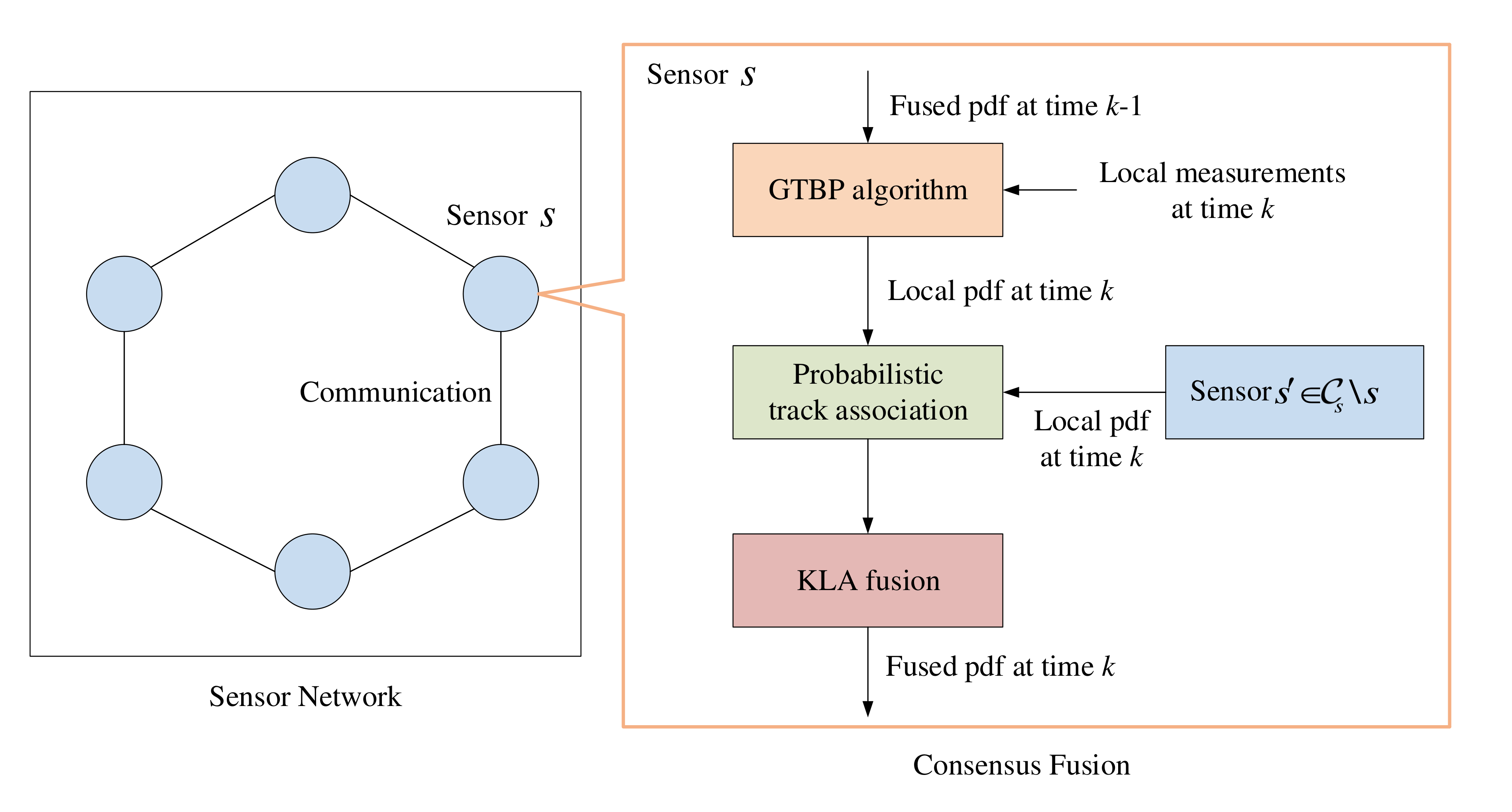
In this paper, we consider solving these problems within the BP framework, where the flowchart of the proposed method is shown in Figure 1. Specifically, for each sensor in the DSN, the GTBP method is used to track the group targets locally and then obtains the local posterior pdf [32]. After exchanging the information between sensors and their neighbors, the track association problem is formulated by a FG and we obtain the track association probabilities by running BP. Finally, the KLA fusion is performed iteratively at each sensor according to the received local posterior pdfs from its neighbors and corresponding track association probabilities. Notably, our proposed method for DGTT using limited FoV sensors does not rely on any specific local tracker, other GTT methods can also be used. Details of the proposed DGTT method are presented in the following subsections.

Figure 1 The flow of the proposed DGTT method.

3.2 Track Association and Consensus Fusion

For simplicity, let us consider the track association between two sensors and the consensus fusion at sensor 1 (reference sensor), which receives the local pdfs from sensor 2 (neighboring sensor). Note that under the setting of limited FoVs of sensors, the KLA fusion rule cannot preserve the information difference and tends to discard the targets located outside the overlapping FoV [16]. To address this issue, we consider dynamically introducing the undetected targets inside the FoV (UTIF) and new targets outside of the FoV (NTOF) of the reference sensor. Specifically, subsections 3.2.1-3.2.2 propose the track association and consensus fusion between the targets inside the FoV of the reference sensor, and subsection 3.2.3 presents the consensus fusion for targets outside the FoV of the reference sensor.

3.2.1 Probabilistic Consensus Fusion

In this subsection, we mainly consider the fusion between the targets inside the FoV of sensor 1. According to the FoV of sensor 1, the targets of its own and received from sensor 2 can be divided into two disjoint sets (i.e., inside or outside the FoV of sensor 1), respectively. We denote $\mathcal{I}_{k,s}:=\{1,\ldots,n_{k,s}\},s=1,2$ as the index sets of targets at sensor $s$ that are inside the FoV of sensor 1, and the corresponding local posterior pdfs are denoted as $p(\mathbf{y}_{k,s}|\mathbf{z}_{1:k,s})$ , where $n_{k,s}$ is the corresponding number of targets. Similar to the introduction of new PTs at local sensors, the UTIF at sensor 1 are modeled by introducing $n_{k,2}$ new PTs (that may be available from sensor 2), i.e., $\overline{\overline{\mathbf{y}}}_{k,1}:=[\overline{\overline{\mathbf{y}}}_{k,1% }^{(1)\mathrm{T}},\ldots,\overline{\overline{\mathbf{y}}}_{k,1}^{(n_{k,2})% \mathrm{T}}]^{\mathrm{T}}$ . Let $\breve{\mathbf{y}}_{k,1}:=[\mathbf{y}_{k,1}^{\mathrm{T}},\overline{\overline{% \mathbf{y}}}_{k,1}^{\mathrm{T}}]^{\mathrm{T}}$ denote the joint augmented state at sensor 1 to be fused, and $\breve{\mathcal{I}}_{k,1}:=\{1,\ldots,\breve{n}_{k,1}\}$ denote the corresponding index set of targets, where $\breve{n}_{k,1}:=n_{k,1}+n_{k,2}$ . Herein, the target indices are ordered, i.e., $\breve{\mathbf{y}}_{k,1}^{(i)},i\in\breve{\mathcal{I}}_{k,1}$ corresponds to the original target $\mathbf{y}_{k,1}^{(i)}$ (at sensor 1) for $i\leq n_{k,1}$ , or the introduced new PT $\overline{\overline{\mathbf{y}}}_{k,1}^{(i-n_{k,1})}$ for $i>n_{k,1}$ .

The track association between sensors 1 and 2 is described by an association vector $\tau:=[\tau^{(1)},\ldots,\tau^{(\breve{n}_{k,1})}]^{\mathrm{T}}$ for sensor 1, where the entries $\tau^{(i)},i\in\mathcal{I}_{k,1}$ are defined as

\displaystyle\tau^{(i)}:=\begin{cases}j\in\mathcal{I}_{k,2},&\begin{array}[]{l% }\text{if }\mathbf{x}_{k,1}^{(i)}\text{ at sensor 1 and }\mathbf{x}_{k,2}^{(j)% }\text{ at}\\ \text{sensor 2 indicate the same target}\end{array}\\ 0,&\begin{array}[]{l}\text{if the target indicated by }\mathbf{x}_{k,1}^{(i)}% \text{ is }\\ \text{undetected by sensor 2,}\end{array}\end{cases}

and for the introduced new PT $i\in\breve{\mathcal{I}}_{k,1}\backslash\mathcal{I}_{k,1}$ , $\tau^{(i)}:=j$ if the target indicated $\mathbf{x}_{k,2}^{(j)},j\in\mathcal{I}_{k,2}$ at sensor 2 is the UTIF at sensor 1. Otherwise, $\tau^{(i)}=0$ , which means the target $\mathbf{x}_{k,1}^{(i)}$ does not exist. Analogously, it is assumed that a PT at sensor 1 can be associated with at most one PT at sensor 2, and vice versa. We denote $\mathcal{T}_{c}$ and $\mathcal{T}$ as the set of all possible $\tau$ and its subset satisfying the constraint, respectively. Let $\mathbf{y}_{k,2}^{\tau}:=[\mathbf{y}_{k,2}^{(\tau^{(1)})\mathrm{T}},\ldots,% \mathbf{y}_{k,2}^{(\tau^{(\breve{n}_{k,1})})\mathrm{T}}]^{\mathrm{T}}$ be the reordered vector of $\mathbf{y}_{k,2}$ according to $\tau$ . Note that $\mathbf{y}_{k,2}^{(0)}$ is the dummy state introduced for the indices $i$ with $\tau^{(i)}=0$ , and thus $\mathbf{y}_{k,2}^{\tau}$ has matched dimension with $\breve{\mathbf{y}}_{k,1}$ . Then, the KLA fusion rule with given $\tau$ for sensors 1 and 2 can be rewritten as

\displaystyle\begin{split}p^{\tau}(\breve{\mathbf{y}}_{k,1}|\mathbf{z}_{1:k,1}% ,\mathbf{z}_{1:k,2})&=\frac{\big{(}p_{1}(\breve{\mathbf{y}}_{k,1})\big{)}^{\pi% _{1}}\big{(}p_{2}(\mathbf{y}_{k,2}^{\tau})\big{)}^{\pi_{2}}}{C_{\tau}}\end{split}

where $\pi_{1}+\pi_{2}=1$ , the pdf $p_{s}(\mathbf{y}_{k,s})$ is short for $p(\mathbf{y}_{k,s}|\mathbf{z}_{1:k,s})$ of sensor $s$ , and the coefficient $C_{\tau}\in[0,1]$ is given by

\displaystyle\begin{split}C_{\tau}:=\int\big{(}p_{1}(\breve{\mathbf{y}}_{k,1})% \big{)}^{\pi_{1}}\big{(}p_{2}(\mathbf{y}_{k,2}^{\tau})\big{)}^{\pi_{2}}\mathrm% {d}{\breve{\mathbf{y}}_{k,1}}=\prod_{i\in\breve{\mathcal{I}}_{k,1}}C_{i,\tau^{% (i)}}\end{split}

where $C_{i,\tau^{(i)}}:=\int\big{(}p_{1}(\breve{\mathbf{y}}_{k,1}^{(i)})\big{)}^{\pi% _{1}}\big{(}p_{2}(\mathbf{y}_{k,2}^{(\tau^{(i)})})\big{)}^{\pi_{2}}\mathrm{d}{% \breve{\mathbf{y}}_{k,1}^{(i)}}$ . Note that $p_{s}(\mathbf{y}_{k,s}^{(i)})=p(\mathbf{x}_{k,s}^{(i)}|r_{k,s}^{(i)},\mathbf{z% }_{1:k,s})p(r_{k,s}^{(i)}|\mathbf{z}_{1:k,s})$ , and if $r_{k,s}^{(i)}=1$ , we abbreviate $p(\mathbf{x}_{k,s}^{(i)}|r_{k,s}^{(i)},\mathbf{z}_{1:k,s})$ and $p(r_{k,s}^{(i)}|\mathbf{z}_{1:k,s})$ as $p_{s}(\mathbf{x}_{k,s}^{(i)})$ and $p_{s}(r_{k,s}^{(i)})$ , respectively. Here, the pdf $p(\mathbf{x}_{k,s}^{(i)}|r_{k,s}^{(i)},\mathbf{z}_{1:k,s})$ represents the dummy pdf when $r_{k,s}^{(i)}=0$ . We denote $p_{\pi}^{i,\tau^{(i)}}(\breve{\mathbf{y}}_{k,1}^{(i)})$ as

\displaystyle\begin{split}&p_{\pi}^{i,\tau^{(i)}}(\breve{\mathbf{x}}_{k,1}^{(i% )},\breve{r}_{k,1}^{(i)}=1):=\\ &\frac{\big{(}p_{1}(\breve{\mathbf{x}}_{k,1}^{(i)})p_{1}(\breve{r}_{k,1}^{(i)}% =1)\big{)}^{\pi_{1}}\big{(}p_{2}(\mathbf{x}_{k,2}^{(\tau^{(i)})})p_{2}(r_{k,2}% ^{(\tau^{(i)})}=1)\big{)}^{\pi_{2}}}{C_{i,\tau^{(i)}}}\\ &=\frac{p_{\pi}^{i,\tau^{(i)}}(\breve{r}_{k,1}^{(i)}=1)p_{\pi}^{i,\tau^{(i)}}(% \breve{\mathbf{x}}_{k,1}^{(i)})}{C_{i,\tau^{(i)}}}\end{split}

with

\displaystyle\begin{split}&p_{\pi}^{i,\tau^{(i)}}(\breve{r}_{k,1}^{(i)}=1)=% \big{(}p_{1}(\breve{r}_{k,1}^{(i)}=1)\big{)}^{\pi_{1}}\big{(}p_{2}(r_{k,2}^{(% \tau^{(i)})}=1)\big{)}^{\pi_{2}}\\ &p_{\pi}^{i,\tau^{(i)}}(\breve{\mathbf{x}}_{k,1}^{(i)})=\big{(}p_{1}(\breve{% \mathbf{x}}_{k,1}^{(i)})\big{)}^{\pi_{1}}\big{(}p_{2}(\mathbf{x}_{k,2}^{(\tau^% {(i)})})\big{)}^{\pi_{2}}\end{split}

and $C_{i,\tau^{(i)}}$ can be rewritten as

\displaystyle\begin{split}C_{i,\tau^{(i)}}&=p_{\pi}^{i,\tau^{(i)}}(\breve{r}_{% k,1}^{(i)}=0)\\ &\quad+p_{\pi}^{i,\tau^{(i)}}(\breve{r}_{k,1}^{(i)}=1)\int p_{\pi}^{i,\tau^{(i% )}}(\breve{\mathbf{x}}_{k,1}^{(i)})\mathrm{d}{\breve{\mathbf{x}}_{k,1}^{(i)}}% \end{split}

Thus, Equation (1) can be rewritten as

\displaystyle\begin{split}p^{\tau}(\breve{\mathbf{y}}_{k,1}|\mathbf{z}_{1:k,1}% ,\mathbf{z}_{1:k,2})=\prod_{i\in\breve{\mathcal{I}}_{k,1}}p_{\pi}^{i,\tau^{(i)% }}(\breve{\mathbf{y}}_{k,1}^{(i)})\end{split}

Notably, the coefficient $C_{\tau}$ can be used for measuring of similarity between the local densities to be fused. Under given $\tau$ , the larger is the coefficient $C_{\tau}$ among the local densities, the more the corresponding KLA fusion is coherent with the Principle of Minimum Discrimination of Information. Thus, given local densities to be fused, different track association vectors $\tau$ result in different coefficients, and a larger $C_{\tau}$ indicates that the corresponding track association vector $\tau$ is more likely. Based on this motivation, we consider the track association problem in a probabilistic way, where the track association vector $\tau$ is random and the pmf of $\tau$ is defined as

\displaystyle p(\tau):=\begin{cases}\alpha C_{\tau},&\begin{array}[]{l}\text{% if }\tau\in\mathcal{T}\end{array}\\ 0,&\begin{array}[]{l}\text{otherwise,}\end{array}\end{cases}

where $\alpha:=1/\sum_{\tau\in\mathcal{T}}C_{\tau}$ . Consequently, the fused posterior pdf $p(\breve{\mathbf{y}}_{k,1}|\mathbf{z}_{1:k,1},\mathbf{z}_{1:k,2})$ is obtained by

\displaystyle\begin{split}p(\breve{\mathbf{y}}_{k,1}|\mathbf{z}_{1:k,1},% \mathbf{z}_{1:k,2})&=\sum_{\tau\in\mathcal{T}}p(\breve{\mathbf{y}}_{k,1},\tau|% \mathbf{z}_{1:k,1},\mathbf{z}_{1:k,2})\\ &=\sum_{\tau\in\mathcal{T}_{c}}p(\breve{\mathbf{y}}_{k,1}|\tau,\mathbf{z}_{1:k% ,1},\mathbf{z}_{1:k,2})p(\tau)\end{split}

where $p(\breve{\mathbf{y}}_{k,1}|\tau,\mathbf{z}_{1:k,1},\mathbf{z}_{1:k,2}):=p^{% \tau}(\breve{\mathbf{y}}_{k,1}|\mathbf{z}_{1:k,1},\mathbf{z}_{1:k,2})$ is the conditional fused posterior pdf. The second equality uses the definition that $p(\tau)=0$ if $\tau\in\mathcal{T}_{c}\backslash\mathcal{T}$ . Similar to [28], we use the product of the marginal pmfs of $p(\tau)$ to approximate the pmf $p(\tau)$ , i.e.,

\displaystyle p(\tau)\approx\prod_{i\in\breve{\mathcal{I}}_{k,1}}\widetilde{p}% (\tau^{(i)}),\quad\tau\in\mathcal{T}_{c}

where $\widetilde{p}(\tau^{(i)}):=\int p(\tau)\mathrm{d}{(\tau\backslash\tau^{(i)})}$ denotes the marginal pmf of the track association vector $\tau$ . Thus, the fused posterior pdf $p(\breve{\mathbf{y}}_{k,1}|\mathbf{z}_{1:k,1},\mathbf{z}_{k,2})$ is approximated by

\displaystyle\begin{split}&p(\breve{\mathbf{y}}_{k,1}|\mathbf{z}_{1:k,1},% \mathbf{z}_{1:k,2})\approx\sum_{\tau\in\mathcal{T}_{c}}\prod_{i\in\breve{% \mathcal{I}}_{k,1}}\widetilde{p}(\tau^{(i)})p_{\pi}^{i,\tau^{(i)}}(\breve{% \mathbf{y}}_{k,1}^{(i)})\\ &=\prod_{i\in\breve{\mathcal{I}}_{k,1}}\sum_{\tau^{(i)}\in\mathcal{I}_{k,2}% \cup\{0\}}\widetilde{p}(\tau^{(i)})p_{\pi}^{i,\tau^{(i)}}(\breve{\mathbf{y}}_{% k,1}^{(i)})=\prod_{i\in\breve{\mathcal{I}}_{k,1}}\widetilde{p}_{\pi}(\breve{% \mathbf{y}}_{k,1}^{(i)})\end{split}

with $\widetilde{p}_{\pi}(\breve{\mathbf{y}}_{k,1}^{(i)})=\sum_{\tau^{(i)}\in% \mathcal{I}_{k,2}\cup\{0\}}\widetilde{p}(\tau^{(i)})p_{\pi}^{i,\tau^{(i)}}(% \breve{\mathbf{y}}_{k,1}^{(i)})$ , and the second equality uses the fact that

\displaystyle\sum\limits_{\tau\in\mathcal{T}_{c}}=\sum\limits_{\tau^{(i)}\in% \mathcal{I}_{k,2}\cup\{0\}}\cdots\sum\limits_{\tau^{(\breve{n}_{k,1})}\in% \mathcal{I}_{k,2}\cup\{0\}}

.

Notably, the original KLA fusion rule tends to retain only targets that exist in all the local posteriors over the network, which makes it unsuitable for the distributed fusion under sensors with limited and different FoVs. Equation (7) provides a probabilistic way to calculate the fused density, where the information difference among sensors is preserved.

Since the knowledge of UTIF is unknown at sensor 1, we construct the prior pdf of UTIF as follows. Let $\mathcal{J}_{k,2}:=\{j:\exists\ i\in\breve{\mathcal{I}}_{k,1}\backslash% \mathcal{I}_{k,1},\ \tau^{(i)}=j\in\mathcal{I}_{k,2},\ 1_{FOV_{1}}(\mathbf{x}_% {k,2}^{(j)})=1\}$ denote the index set of targets at sensor 2 that are UTIF of sensor 1, the pdf $p(\breve{\mathbf{x}}_{k,1}^{(i)}|\mathbf{z}_{k,1})$ is given by the following Gaussian mixture model

\displaystyle p(\breve{\mathbf{x}}_{k,1}^{(i)}|\mathbf{z}_{k,1}):=\frac{1}{|% \mathcal{J}_{k,2}|}\sum_{j\in\mathcal{J}_{k,2}}\mathcal{N}(\breve{\mathbf{x}}_% {k,1}^{(i)};\mathbb{E}[\mathbf{x}_{k,2}^{(j)}],\mathbf{P})

where $\mathbb{E}[\cdot]$ is the expectation operator, and $\mathbf{P}$ is a prior covariance. The existence probability of UTIF is a parameter, which may be set to a value related to the detection ability of sensor 1 and the existence probability of the corresponding PT received from sensor 2. Furthermore, if the new PT $i\in\breve{\mathcal{I}}_{k,1}\backslash\mathcal{I}_{k,1}$ at sensor 1 is matched with a dummy PT at sensor 2 (i.e., $\tau^{(i)}=0$ ), then it does not exist and is represented by a dummy pdf $f_{\mathrm{D}}(\breve{\mathbf{x}}_{k,1}^{(i)})$ .

3.2.2 BP-based Track Association

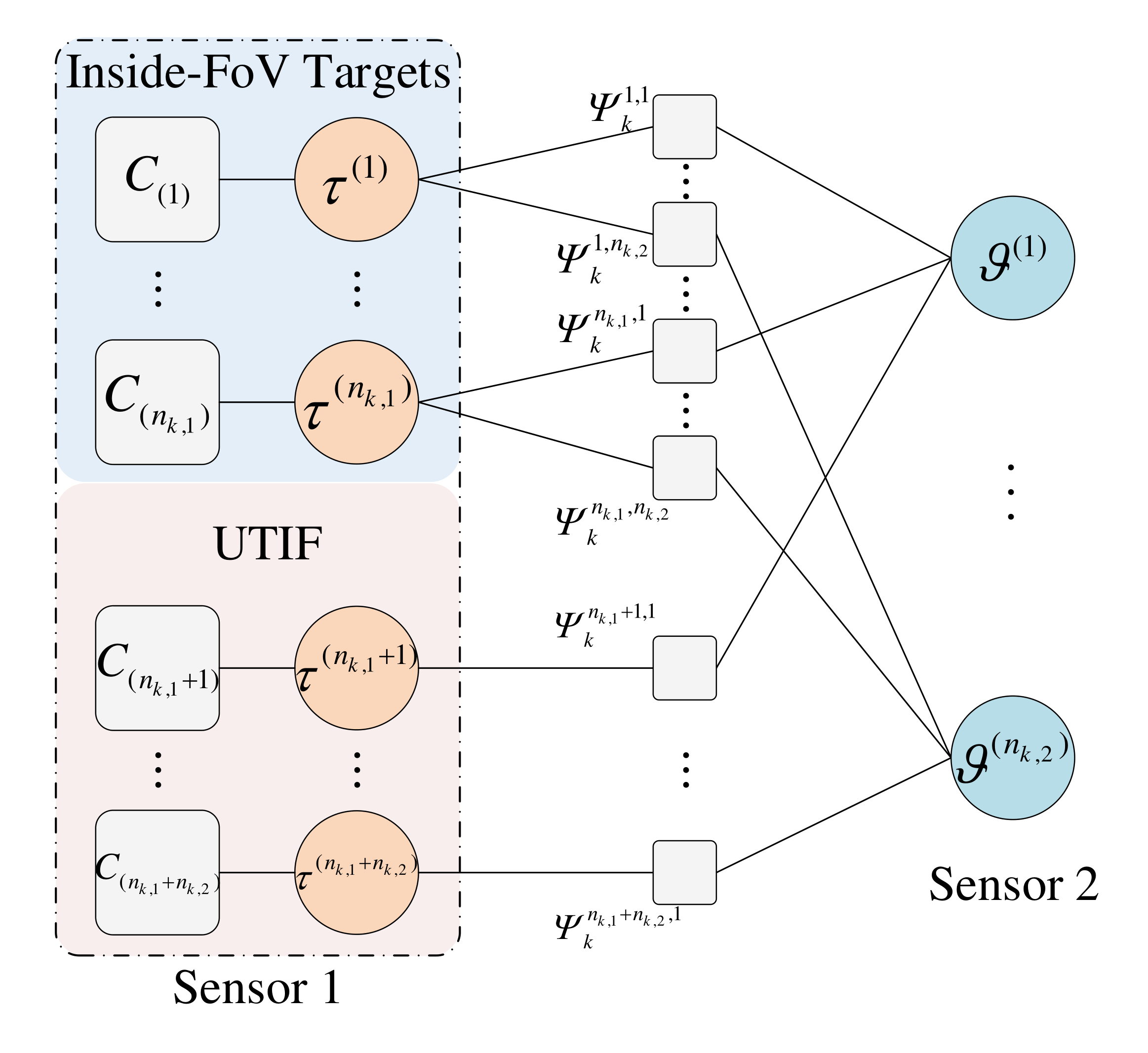
To perform the probabilistic fusion rule (7), it is necessary to calculate marginal pmfs of $p(\tau)$ . In this subsection, we obtain the approximate marginal pmfs of $p(\tau)$ by running BP on the FG devised for track association. According to (5), we have

\displaystyle p(\tau)\propto\varPsi(\tau)\prod_{i\in\breve{\mathcal{I}}_{k,1}}% C_{i,\tau^{(i)}},\quad\tau\in\mathcal{T}_{c}

where $\varPsi(\tau)=1$ if $\tau\in\mathcal{T}$ and $\varPsi(\tau)=0$ otherwise. Similarly, we introduce the association vector $\vartheta:=\left[\vartheta^{(1)},\ldots,\vartheta^{(n_{k,2})}\right]^{\mathrm{% T}}$ for sensor 2, where the entries $\vartheta^{(j)}\in\mathcal{I}_{k,1}\cup\{0\}$ . Herein, we make convention that $\vartheta^{(j)}=0$ means that the target indicated by $\mathbf{x}_{k,2}^{(j)}$ at sensor 2 is the UTIF at sensor 1, i.e., $\tau^{(n_{k,1}+j)}=j$ . The association vector $\vartheta$ for sensor 2 is redundant with $\tau$ for sensor 1, that is, one of the two association vectors is determined and the other is determined as well. By introducing $\vartheta$ , $\varPsi(\tau)$ can be stretched and equivalently expressed as

\displaystyle\varPsi(\tau,\vartheta):=\big{(}\prod_{i\in\mathcal{I}_{k,1}}% \prod_{j\in\mathcal{I}_{k,2}}\varPsi_{k}^{i,j}\big{)}\prod_{i^{\prime}\in% \breve{\mathcal{I}}_{k,1}\backslash\mathcal{I}_{k,1}}\varPsi_{k}^{i^{\prime},1}

where

\displaystyle\varPsi_{k}^{i,j}:=\begin{cases}0,&\begin{array}[]{l}\tau^{(i)}=j% ,\ \vartheta^{(j)}\neq i\text{ or }\vartheta^{(j)}=i,\ \tau^{(i)}\neq j\end{% array}\\ 1,&\begin{array}[]{l}\text{otherwise, }\end{array}\end{cases}

\displaystyle\varPsi_{k}^{i^{\prime},1}:=\begin{cases}0,&\begin{array}[]{l}% \tau^{(i^{\prime})}=i^{\prime}-n_{k,1},\ \vartheta^{(i^{\prime}-n_{k,1})}\neq 0% \text{ or }\\ \vartheta^{(i^{\prime}-n_{k,1})}=0,\ \tau^{(i^{\prime})}\neq i^{\prime}-n_{k,1% }\end{array}\\ 1,&\begin{array}[]{l}\text{otherwise. }\end{array}\end{cases}

Thus, the pmf $p(\tau)$ in (9) can be rewritten as

\displaystyle p(\tau,\vartheta)\propto\big{(}\prod_{i\in\mathcal{I}_{k,1}}C_{i% ,\tau^{(i)}}\prod_{j\in\mathcal{I}_{k,2}}\varPsi_{k}^{i,j}\big{)}\prod_{i^{% \prime}\in\breve{\mathcal{I}}_{k,1}\backslash\mathcal{I}_{k,1}}C_{i,\tau^{(i)}% }\varPsi_{k}^{i^{\prime},1}

A FG representation of the factorization (10) is shown in Figure 2, which enables the use of efficient BP scheme for the track association problem.

Figure 2 Factor graph representation for the factorization of

p(\tau,\vartheta)

in (10). Herein,

C_{(i)}

is short for

C_{i,\tau^{(i)}},i\in\breve{\mathcal{I}}_{k,1}

Specifically, once the incoming messages $C_{i,\tau^{(i)}}$ to the track association part have been calculated, the iterative message calculation between $\tau^{(i)}$ , $\vartheta^{(j)}$ and $\varPsi_{k}^{i,j}$ are performed. In the iteration, the messages $\varphi_{\varPsi_{k}^{i,j}\rightarrow\vartheta^{(j)}}^{\left[\ell\right]}(% \vartheta^{(j)})$ , and $\phi_{\varPsi_{k}^{i,j}\rightarrow\tau^{(i)}}^{\left[\ell\right]}(\tau^{(i)})$ are iteratively updated, where the superscript $\ell$ denotes the number of iterations. Hereafter, we abbreviate them as $\varphi_{i\rightarrow j}^{\left[\ell\right]}$ and $\phi_{j\rightarrow i}^{\left[\ell\right]}$ for notational convenience. The calculation of $\varphi_{i\rightarrow j}^{\left[\ell\right]}$ for $i\in\mathcal{I}_{k,1}$ and $j\in\mathcal{I}_{k,2}$ are given by

\displaystyle\begin{split}\varphi_{i\rightarrow j}^{\left[\ell\right]}=\sum_{% \tau^{(i)}\in\mathcal{I}_{k,2}\cup\{0\}}C_{i,\tau^{(i)}}\varPsi_{k}^{i,j}\prod% _{j^{\prime}\in\mathcal{I}_{k,2}\backslash j}\phi_{j^{\prime}\rightarrow i}^{% \left[\ell\right]}\end{split}

and $\varphi_{i\rightarrow j}^{\left[\ell\right]}=\sum_{\tau^{(i)}\in\{0,j\}}C_{i,% \tau^{(i)}}\varPsi_{k}^{i,1}$ with $j=i-n_{k,1}$ for $i\in\breve{\mathcal{I}}_{k,1}\backslash\mathcal{I}_{k,1}$ . Similarly, the messages $\phi_{j\rightarrow i}^{\left[\ell\right]}$ for $j\in\mathcal{I}_{k,2}$ and $i\in\mathcal{I}_{k,1}$ are computed by

\displaystyle\begin{split}\phi_{j\rightarrow i}^{\left[\ell\right]}=\sum_{% \vartheta^{(j)}\in\mathcal{I}_{k,1}\cup\{0\}}\varPsi_{k}^{i,j}\varphi_{n_{k,1}% +j\rightarrow j}^{\left[\ell-1\right]}\prod_{{i^{\prime}\in\mathcal{I}_{k,1}% \backslash i}}\varphi_{i^{\prime}\rightarrow j}^{\left[\ell-1\right]}\end{split}

and $\phi_{j\rightarrow i}^{\left[\ell\right]}=\sum_{\vartheta^{(j)}\in\mathcal{I}_% {k,1}\cup\{0\}}\varPsi_{k}^{i,1}\prod_{i^{\prime}\in\mathcal{I}_{k,1}}\varphi_% {i^{\prime}\rightarrow j}^{\left[\ell-1\right]}$ with $i=n_{k,1}+j$ for $j\in\mathcal{I}_{k,2}$ . The iterative loop of (11)-(12) is initialized by setting

\displaystyle\begin{split}\varphi_{i\rightarrow j}^{\left[0\right]}=&\sum_{% \tau^{(i)}\in\mathcal{I}_{k,2}\cup\{0\}}C_{i,\tau^{(i)}}\varPsi_{k}^{i,j},\ i% \in\mathcal{I}_{k,1}\\ \varphi_{i\rightarrow i-n_{k,1}}^{\left[0\right]}=&\sum_{\tau^{(i)}\in\{0,i-n_% {k,1}\}}C_{i,\tau^{(i)}}\varPsi_{k}^{i,1},\ i\in\breve{\mathcal{I}}_{k,1}% \backslash\mathcal{I}_{k,1}\end{split}

The implementation and termination of the iteration (11)-(12) is analogous to the iteration data association at local sensors [32]. We denote the number of iterations when meeting the stopping criteria as $L_{T}$ , then the beliefs $\widetilde{p}(\tau^{(i)}=j)$ approximating the marginal pmfs of $p(\tau)$ are obtained as

\displaystyle\widetilde{p}(\tau^{(i)}=j)=\frac{C_{i,j}\phi_{j\rightarrow i}^{% \left[L_{T}\right]}}{\sum_{j^{\prime}\in\mathcal{I}_{k,2}\cup\{0\}}C_{i,j^{% \prime}}\phi_{j^{\prime}\rightarrow i}^{\left[L_{T}\right]}}

with $\phi_{0\rightarrow i}^{\left[L_{T}\right]}:=1$ for $i\in\mathcal{I}_{k,1}$ and $j\in\mathcal{I}_{k,2}\cup\{0\}$ , and

\displaystyle\widetilde{p}(\tau^{(i)}=j):=\begin{cases}\frac{C_{i,j}\phi_{j% \rightarrow i}^{\left[L_{T}\right]}}{C_{i,0}+C_{i,j}\phi_{j\rightarrow i}^{% \left[L_{T}\right]}},&\begin{array}[]{l}j=i-n_{k,1}\end{array}\\ \frac{C_{i,0}}{C_{i,0}+C_{i,j}\phi_{j\rightarrow i}^{\left[L_{T}\right]}},&% \begin{array}[]{l}j=0,\end{array}\end{cases}

for $i\in\breve{\mathcal{I}}_{k,1}\backslash\mathcal{I}_{k,1}$ . We summarize the BP-based probabilistic track association algorithm as follows:

Algorithm 1 BP-based Probabilistic Track Association

Input: Local pdfs

p_{1}(\mathbf{y}_{k,1})

and

p_{2}(\mathbf{y}_{k,2})

from sensors 1 and 2, respectively; Output: Beliefs

\widetilde{p}(\tau^{(i)})

i\in\breve{\mathcal{I}}_{k,1}

j\in\mathcal{I}_{k,2}\cup\{0\}

;

According to (4) and (8), compute the messages $C_{i,\tau^{(i)}}$ by using local pdfs;
Initialize $\varphi_{i\rightarrow j}^{\left[0\right]}$ by (13), and iteratively compute the messages $\phi_{j\rightarrow i}^{\left[\ell\right]}$ , $\varphi_{i\rightarrow j}^{\left[\ell\right]}$ for $\ell=1,\ldots,L_{T}$ ;
Compute the beliefs $\widetilde{p}(\tau^{(i)})$ via (14) and (15);
return the beliefs $\widetilde{p}(\tau^{(i)})$ , $i\in\breve{\mathcal{I}}_{k,1}$ , $j\in\mathcal{I}_{k,2}\cup\{0\}$ ;

3.2.3 Consensus Fusion for Outside-FoV Targets

Let $\mathcal{M}_{k,s},s=1,2$ denote the index sets of targets at sensor $s$ , which are outside the FoV of the reference sensor 1. We present the fusion scheme for targets $\mathcal{M}_{k,1}$ and $\mathcal{M}_{k,2}$ that are outside the FoV of the reference sensor 1 as follows.

Step 1: For each target $i\in\mathcal{M}_{k,1}$ (maintained at sensor 1) that received from sensor 2 at the previous time step, update it by corresponding new information received from sensor 2 at the current time step.
Step 2: For the rest of targets (in $\mathcal{M}_{k,1}$ ) at sensor 1, perform the track association and consensus fusion with the rest of targets (in $\mathcal{M}_{k,2}$ ) received from sensor 2 (as described in subsections 3.2.1-3.2.2).
Step 3: For the unmatched targets (in $\mathcal{M}_{k,2}$ ) received from sensor 2, maintain them at sensor 1.

3.3 Summary of the Proposed DGTT Method

As presented before, Equation (7) provides the fusion rule for two sensors in a probabilistic way, where the track association problem can be efficiently solved by running BP on the devised FG. While in practical distributed fusion system with multi-sensor, it is often that more than two local posterior pdfs to be fused and a common method is to perform the pairwise fusion. Thus, the fusion of $|\mathcal{C}_{s}|>2$ sensors can be implemented by sequentially using the BP-based track association method and the pairwise fusion (7) $|\mathcal{C}_{s}|-1$ times. Specific procedure is summarized in Algorithm 2.

Algorithm 2 Consensus Fusion Algorithm

Input:

|\mathcal{C}_{s}|

local pdfs to be fused at sensor

s\in\mathcal{S}

; Output: The fused pdf at sensor

s

;

for $s^{\prime}\in\mathcal{C}_{s}\backslash s$ do
Divide the targets at sensors $s$ and $s^{\prime}$ into two disjoint sets according to the FoV of sensor $s$ , respectively;
For the targets at sensors $s$ and $s^{\prime}$ that are inside the FoV of sensor $s$ , compute the marginal track association probabilities by Algorithm 1 using local pdfs (at sensors $s$ and $s^{\prime}$ ), and compute the fused pdf at sensor $s$ via (7);
For the targets at sensors $s$ and $s^{\prime}$ that are outside the FoV of sensor $s$ , performing the consensus fusion scheme as described in subsection 3.2.3;
Substitute the fused pdf for the local pdf at sensor $s$ ;
end for
return the fused pdf at sensor $s$ ;

Thus, the main steps of the overall DGTBP algorithm is concluded as follows:

GTBP for local sensors: Each local sensor $s\in\mathcal{S}$ receives the local measurements $\mathbf{z}_{k,s}$ at time $k$ , and runs GTBP [32] to obtain the local posterior pdf;
Iterative consensus fusion for each local sensor: After the processing of local sensors, $L_{C}$ consensus iterations are performed over the DSN. In each iteration, each sensor $s$ receives the local pdfs from its neighboring sensors $s^{\prime}\in\mathcal{C}_{s}\backslash s$ . After the information exchange, each sensor $s$ performs the consensus-based fusion via Algorithm 2. Note that the original local posterior pdf at each sensor $s$ is replaced by corresponding fused pdf after running Algorithm 2, which is used in the next consensus iteration.
State estimation and pruning: After performing $L_{C}$ consensus iterations, the state estimations and existence probabilities are obtained for each sensor $s\in\mathcal{S}$ through the corresponding fused pdf. Finally, a pruning step is performed at each local sensor to remove unlikely PTs based on the existence probabilities.

3.4 Computational Complexity and Scalability

By exploiting the scalability of BP, we propose a DGTBP method. For ease of representation, we analyze the computational complexity of DGTBP under the assumption of a fixed number of BP iterations, and we use the maximum possible number of PTs $N_{\text{max}}:=\max\{N_{1},\ldots,N_{S}\}$ appearing in the DSN to analyze how the computational complexity scales in the number of PTs. In fact, this upper bound $N_{\text{max}}$ will not be reached in most cases due to the FoV limitations. Specifically, for each sensor $s\in\mathcal{S}$ , the overall computational complexity mainly contains the following two parts:

The computational complexity of GTBP: As shown in [32], the prediction of the group structure requires to be computed $|\underline{\mathcal{G}}_{k,s}|$ times, that is, its computational complexity scales as $\mathcal{O}(|\underline{\mathcal{G}}_{k,s}|)$ . Furthermore, the computational complexity of the measurement evaluation and iterative data steps association scales as $\mathcal{O}(N_{\text{max}}m_{k,s})$ .
The computational complexity of consensus fusion: Each sensor $s$ requires to perform $|\mathcal{C}_{s}|-1$ times of the pairwise consensus fusion based on Algorithm 2. Thus, the computational complexity of performing consensus fusion at sensor $s$ scales as $\mathcal{O}(|\mathcal{C}_{s}|)$ . Since the maximum possible number of PTs is $N_{\text{max}}$ , the computational complexity of (4), (11), and (12) scales as $\mathcal{O}(N_{\text{max}}^{2})$ in each pairwise fusion.

Thus, the overall computational complexity of DGTBP at each sensor $s\in\mathcal{S}$ scales linearly in the numbers of group partitions, local measurements, and its neighboring sensors, and quadratically in the number of PTs.

.

Notably, the computational complexity can be further reduced in different ways, e.g., gating preprocessing of targets and measurements [5], censoring of messages [29], preserving the $M$ -best group partitions, etc. Specifically, gating technology can be employed for keeping the number of considered group partitions and the size of iterative data association at a tractable level. Message censoring ignores these messages related to new PTs that are unlikely to be an actual target. Preserving the $M$ -best group partitions at each time step reduces the computational complexity of calculating the messages that involve the summation over possible group partitions.

4. Algorithm Implementation

For the suitability of general nonlinear and non-Gaussian dynamic system, we consider the Monte Carlo (MC) implementation of the proposed DGTBP method in this section. Due to limited space, we mainly present the details of the particle-based probabilistic track association and consensus fusion (i.e., step 3 in Algorithm 2), where the particle implementation of $M$ -best GTBP for local sensors is provided in [32].

Let $\{\{(\mathbf{x}_{k,s}^{(i,l)},w_{k,s}^{(i,l)})\}_{l=1}^{L_{s}}\}_{i=1}^{n_{k,s}}$ denote the particle representation of the belief $\widetilde{p}(\mathbf{x}_{k,s},\mathbf{r}_{k,s})$ approximating the local posterior pdf $p_{s}(\mathbf{y}_{k,s})$ , $s\in\{1,2\}$ , where $L_{s}$ is the number of particles. Note that the summation $\sum_{l=1}^{L_{s}}w_{k,s}^{(i,l)}$ provides an approximation of the marginal posterior pmf $p_{s}(r_{k,s}^{(i)}=1)$ . Before performing the consensus fusion (7), the beliefs $\widetilde{p}(\tau^{(i)})$ and the pdfs $p_{\pi}^{i,\tau^{(i)}}(\breve{\mathbf{y}}_{k,1}^{(i)})$ are required to be computed. However, since each sensor has its own particle-based implementation with its own support, the particle representation of the fused pdf cannot be directly computed. A natural and common way is to use the union of the particles as the support, and adopt the kernel density estimation (KDE) method[13]. A KDE approximation of $p_{s}(\mathbf{x}_{k,s}^{(i)})$ is given by

\displaystyle\widetilde{K}_{s}(\mathbf{x}_{k,s}^{(i)}):=\frac{1}{V_{h}}\sum_{l% =1}^{L_{s}}\overline{w}_{k,s}^{(i,l)}K(\frac{\mathbf{x}_{k,s}^{(i)}-\mathbf{x}% _{k,s}^{(i,l)}}{h})

where $\overline{w}_{k,s}^{(i,l)}:=w_{k,s}^{(i,l)}/\sum_{l=1}^{L_{s}}w_{k,s}^{(i,l)}$ , $K(\cdot)$ is a Kernel function, $h$ is the bandwidth, and $V_{h}$ is the volume of $K$ which depends also on $h$ . The use of a Gaussian KDE and corresponding choice of the bandwidth can be seen in [13].

Let $\mathcal{X}_{i,\tau^{(i)}}:=\{\mathbf{x}_{k,1}^{(i,l)}\}_{l=1}^{L_{1}}\cup\{% \mathbf{x}_{k,2}^{(\tau^{(i)},l)}\}_{l=1}^{L_{2}}$ denote the union of the particles11 to represent $p_{\pi}^{i,\tau^{(i)}}(\breve{\mathbf{x}}_{k,1}^{(i)})$ in (3), which can be seen as the samples drawn from the following the mixture important sampling density,

\displaystyle p_{IS}(\mathbf{x}):=\frac{L_{1}\big{(}p_{1}(\breve{\mathbf{x}}_{% k,1}^{(i)}=\mathbf{x})\big{)}^{\pi_{1}}+L_{2}\big{(}p_{2}(\mathbf{x}_{k,2}^{(% \tau^{(i)})}=\mathbf{x})\big{)}^{\pi_{2}}}{L_{1}+L_{2}}

and the weights for particles $\mathbf{x}_{i,\tau^{(i)}}^{(l)}\in\mathcal{X}_{i,\tau^{(i)}}$ are given by

\displaystyle\zeta_{i,\tau^{(i)}}^{(l)}\propto\frac{\big{(}p_{1}(\mathbf{x}_{i% ,\tau^{(i)}}^{(l)})\big{)}^{\pi_{1}}\big{(}p_{2}(\mathbf{x}_{i,\tau^{(i)}}^{(l% )})\big{)}^{\pi_{2}}}{L_{1}\big{(}p_{1}(\mathbf{x}_{i,\tau^{(i)}}^{(l)})\big{)% }^{\pi_{1}}+L_{2}\big{(}p_{2}(\mathbf{x}_{i,\tau^{(i)}}^{(l)})\big{)}^{\pi_{2}}}

By using the KDE approximation (1), the weights can be approximated computed as follows:

\displaystyle\widetilde{\zeta}_{i,\tau^{(i)}}^{(l)}=\widetilde{D}_{\widetilde{% \zeta}_{i,\tau^{(i)}}}^{-1}\frac{\big{(}\widetilde{K}_{1}(\mathbf{x}_{i,\tau^{% (i)}}^{(l)})\big{)}^{\pi_{1}}\big{(}\widetilde{K}_{2}(\mathbf{x}_{i,\tau^{(i)}% }^{(l)})\big{)}^{\pi_{2}}}{L_{1}\big{(}\widetilde{K}_{1}(\mathbf{x}_{i,\tau^{(% i)}}^{(l)})\big{)}^{\pi_{1}}+L_{2}\big{(}\widetilde{K}_{2}(\mathbf{x}_{i,\tau^% {(i)}}^{(l)})\big{)}^{\pi_{2}}}

where $\widetilde{D}_{\widetilde{\zeta}_{i,\tau^{(i)}}}$ is the normalization constant that provides an approximation of the integral of $p_{\pi}^{i,\tau^{(i)}}(\breve{\mathbf{x}}_{k,1}^{(i)})$ ,

\displaystyle\widetilde{D}_{\widetilde{\zeta}_{i,\tau^{(i)}}}\approx\sum_{l=1}% ^{|\mathcal{X}_{i,\tau^{(i)}}|}\frac{\big{(}\widetilde{K}_{1}(\mathbf{x}_{i,% \tau^{(i)}}^{(l)})\big{)}^{\pi_{1}}\big{(}\widetilde{K}_{2}(\mathbf{x}_{i,\tau% ^{(i)}}^{(l)})\big{)}^{\pi_{2}}}{L_{1}\big{(}\widetilde{K}_{1}(\mathbf{x}_{i,% \tau^{(i)}}^{(l)})\big{)}^{\pi_{1}}+L_{2}\big{(}\widetilde{K}_{2}(\mathbf{x}_{% i,\tau^{(i)}}^{(l)})\big{)}^{\pi_{2}}}

The particles $\mathbf{x}_{i,\tau^{(i)}}^{(l)}\in\mathcal{X}_{i,\tau^{(i)}}$ with weights $\widetilde{\zeta}_{i,\tau^{(i)}}^{(l)}$ provide a particle representation of $p_{\pi}^{i,\tau^{(i)}}(\breve{\mathbf{x}}_{k,1}^{(i)})$ . Thus, a particle-based approximation of $C_{i,\tau^{(i)}}$ in (4) is given by

\displaystyle\begin{split}\widetilde{C}_{i,\tau^{(i)}}:=&(1-\sum_{l=1}^{L_{1}}% w_{k,1}^{(i,l)})^{\pi_{1}}(1-\sum_{l=1}^{L_{2}}w_{k,2}^{(\tau^{(i)},l)})^{\pi_% {2}}\\ &+(\sum_{l=1}^{L_{1}}w_{k,1}^{(i,l)})^{\pi_{1}}(\sum_{l=1}^{L_{2}}w_{k,2}^{(% \tau^{(i)},l)})^{\pi_{2}}\widetilde{D}_{\widetilde{\zeta}_{i,\tau^{(i)}}}\end{split}

Substituting $\widetilde{C}_{i,\tau^{(i)}}$ for $C_{i,\tau^{(i)}}$ in (11) and (13), and then the track association between sensors are implemented by running (11)-(12) iteratively. After the iteration terminated, the beliefs $\widetilde{p}(\tau^{(i)})$ approximating the marginal pmfs of $p(\tau)$ are obtained by (14)-(15). Let $\mathcal{X}_{i}:=\cup_{\{\tau^{(i)}:\widetilde{p}(\tau^{(i)})>0\}}\mathcal{X}_% {i,\tau^{(i)}}$ denote the union of the sets of particles with $\widetilde{p}(\tau^{(i)})>0$ . Therefore, the fused posterior pdf $\widetilde{p}_{\pi}(\breve{\mathbf{y}}_{k,1}^{(i)})$ in (7) can be represented by the particles $\{\breve{\mathbf{x}}_{k,1}^{(i,l)}\}_{l=1}^{|\mathcal{X}_{i}|}$ , where each particle $\breve{\mathbf{x}}_{k,1}^{(i,l)}$ equals to one of the particle belonging to $\mathcal{X}_{i}$ , and the corresponding weight is given as follows:

\displaystyle\widetilde{w}_{k,1}^{(i,l)}=\widetilde{p}(\tau^{(i)})\frac{(\sum% \limits_{l^{\prime}=1}^{L_{1}}w_{k,1}^{(i,l^{\prime})})^{\pi_{1}}(\sum\limits_% {l^{\prime}=1}^{L_{2}}w_{k,2}^{(\tau^{(i)},l^{\prime})})^{\pi_{2}}\widetilde{% \zeta}_{i,\tau^{(i)}}^{(l)}}{\widetilde{C}_{i,\tau^{(i)}}}

Next, a resampling step is performed to reduce the $|\mathcal{X}_{i}|$ particles to $L_{1}$ uniformly weighted particles at sensor 1, which are used for the next time of the pairwise fusion.

.

Note that in each consensus iteration, each sensor is required to transmit its own particles to the neighbors of sensors, which may be impractical in the case of limited communication bandwidth. To reduce the communication burden, one may further approximate the particle representation of pdfs at local sensors by Gaussian pdfs. Then, the Gaussian parameters (i.e., mean and covariance) are exchanged between sensors as an alternative [15, 28]. By this way, the consensus fusion are performed by using the collected Gaussian pdfs at each sensor, followed by the conversion of the fused pdfs into particles.

5. Experiments

5.1 Simulation Setting, Comparison Methods and Performance Metrics

We simulate three GTT scenarios using different DSNs of increasing complexity to verify the performance of the proposed method. Specifically,

Scenario 1 simulates two sensor nodes with limited FoVs, merging and splitting group targets, which is applied to validate the capability of handling group splitting and merging of the proposed method.
Scenario 2 simulates multiple sensor nodes with limited FoVs, multiple group targets, and ungrouped targets, which is used for evaluating the tracking performance of the proposed method.
Scenario 3 simulates a large number of sensors with limited FoVs and is used to validate the scalability of DGTBP.

These scenarios are simulated in the 2-D case with 100 time steps and the time sampling interval $\Delta T=2$ s, where the individual targets are described by the state vectors $\mathbf{x}_{k}^{(i)}=[x_{k}^{(i)},\dot{x}_{k}^{(i)},y_{k}^{(i)},\dot{y}_{k}^{(% i)}]^{\mathrm{T}}$ of planar position and velocity. The numbers of group targets and ungrouped targets are time-varying, and the ground truths are simulated using the constant velocity (CV) model and the coordinate turn (CT) model [5]. The target $\mathbf{x}_{k}^{(i)}$ generates a measurement $\mathbf{z}_{k,s}^{(m)}:=[x_{k}^{(i)},y_{k}^{(i)}]^{\mathrm{T}}-\mathbf{p}_{k,s% }+\eta_{k,s}^{(m)}$ by sensor $s$ if and only if $1_{FOV_{s}}(\mathbf{x}_{k}^{(i)})=1$ and it is detected by sensor $s$ , where $\mathbf{p}_{k,s}$ is the location of sensor $s$ at time $k$ and $\mathcal{N}(\eta_{k,s}^{(m)};\mathbf{0},\mathbf{R})$ is a zero-mean Gaussian process noise with $\mathbf{R}=\text{diag}(\sigma_{\eta}^{2},\sigma_{\eta}^{2})$ and $\sigma_{\eta}=10$ m. The clutter pdf $f_{\mathrm{c}}^{(s)}(\mathbf{z}_{k,s}^{(m)})$ is assumed uniform in the FoV of sensor $s$ . Furthermore, we employ the same birth pdf $f_{\mathrm{b}}^{(s)}(\overline{\mathbf{x}}_{k,s}^{(m)})$ constructed by using the measurements at the previous time step [36] for the fair comparison of all tested methods. The Poisson mean numbers of clutter measurements and new PTs for each sensor are set to $\mu_{\mathrm{c}}^{(s)}=1$ and $\mu_{\mathrm{b}}^{(s)}=5\times 10^{-4}$ in these scenarios, respectively.

We consider the particle-based implementation of DGTBP, which adopts the algorithm paradigm in Figure 1 for networks of sensors with limited FoVs. To verify the performance of DGTBP, we compare it with the distributed BP (DBP) method, which can be obtained by employing the same algorithm paradigm as DGTBP with the BP method [23] substituted for GTBP executing at local sensors. Furthermore, we also consider a centralized GTBP (CGTBP) method, which is a generation of the GTBP method [32] to multi-sensor case by using a sensor-sequential processing summarized in [23] (cf. Section IX-B). The results of BP, GTBP for local sensors are provided as well. Due to the settings of limited FoVs, we adopt the following detection probability $p_{\mathrm{d}}^{(s)}(\underline{\mathbf{x}}_{k,s}^{(i)})=W_{k,s}^{(i)}\times P% _{D}$ at any sensor $s$ , where $P_{D}=0.99$ and $W_{k,s}^{(i)}:=\sum_{l=1}^{L_{s}}1_{FOV_{s}}(\mathbf{x}_{k,s}^{(i,l)})w_{k,s}^% {(i,l)}/(\sum_{l=1}^{L_{s}}w_{k,s}^{(i,l)})$ is the summation of normalized weights of these particles inside $FOV_{s}$ . Herein, the coefficient $W_{k,s}^{(i)}$ is used to handle the case that targets move across the boundaries of limited FoVs, which makes the detection probability more adaptive. The number of particles (for representing each legacy PT or new PT state), the survival probability, and the thresholds for target declaration and pruning are set to $L_{s}=1000$ , $p_{\mathrm{e}}^{(s)}(\mathbf{x}_{k}^{(i)})=0.99$ , $P_{\mathrm{c}}=0.8$ , and $P_{\mathrm{pr}}=10^{-3}$ , respectively. In all simulations, a target is pruned if its existence probability is less than $P_{\mathrm{pr}}$ . Since DBP and DGTBP do not require sharing FoV information between sensors, an additional pruning rule is also used for DBP and DGTBP, i.e., a target is pruned if it is not associated with local sensor measurements and other sensors' targets in $K_{\mathrm{pr}}$ consecutive time steps. Furthermore, we use the CV model with the process noise $Q_{\mathrm{CV}}=\sigma_{v}^{2}GG^{\mathrm{T}}$ for filtering, where $\sigma_{v}=3$ m/s² and

\displaystyle G:=\left[\begin{array}[]{cccc}\frac{\Delta T^{2}}{2}&\Delta T&0&% 0\\ 0&0&\frac{\Delta T^{2}}{2}&\Delta T\end{array}\right]^{\mathrm{T}}

In the iterative data association for local trackers and track association between sensors, the iteration is stopped if the difference in the Frobenius norm of the beliefs is less than $10^{-5}$ in two consecutive iterations or reaches the maximum number 100 of iterations. Furthermore, these methods perform message censoring (described in remark 2) with thresholds 0.3 and 0.1 for the data association at local sensors and track association between sensors, respectively. In the implementation of GTBP, 5-best group partitions are preserved at each time step. For DBP and DGTBP, 3 consensus fusion iterations are performed at each time step22. More specifically, in each fusion iteration, the conversion of particles and Gaussian pdfs mentioned in Remark 3 is applied, and only the approximate pdfs of targets with existence probabilities exceeding the threshold $P_{\mathrm{c}}$ for target declaration are transmitted.

To compare the tracking performance, we use the OSPA distance $d_{p}^{(c)}(\cdot,\cdot)$ and the OSPA⁽²⁾ distance $\check{d}_{p,q}^{(c)}(\cdot,\cdot\ ;w)$ as the performance metrics, which is capable of capturing a variety of tracking errors, including location and cardinality errors, track switching and fragmentation [38, 39]. The cutoff parameter, the order parameters, and the window length are set to $c=50$ , $p=1$ , $q=2$ , and $w=10$ (with uniform weights), respectively.

5.2 Scenario 1: Two Nodes with Merging and Splitting Group Targets

Figure 3 The ground truths simulated in scenario 1. Sensor nodes, starting and stopping positions are marked with ✩,

\circ

, and

\square

, respectively.

In scenario 1, we consider tracking an unknown number of group targets with group splitting and merging by using two sensors with limited FoVs. The simulated ground truths, sensor locations, and FoVs are shown in Figure 3. The two sensors are positioned at $[500\ \text{m},\ 3000\ \text{m}]^{\mathrm{T}}$ and $[3200\ \text{m},\ 3000\ \text{m}]^{\mathrm{T}}$ with the radius being 2000 m, respectively. Targets 1, 2, and 3 are born at the time step $k=1$ in the FoV of sensor 1 and then merge into one group and traverse the overlapping FoV. Followed by the group splitting, the three targets die at $k=80$ in the FoV of sensor 2. Moreover, the group targets 4 and 5 are born at $k=11$ and die at $k=90$ in the FoV of sensor 1, respectively. Target 6 is born at $k=21$ in the FoV of sensor 2 and dies at $k=100$ in the FoV of sensor 1. The maximum possible number of PTs is set to $15$ when using CGTBP, and otherwise $10$ . The pruning length threshold is set to $K_{\mathrm{pr}}=2$ in the implementations of DBP and DGTBP.

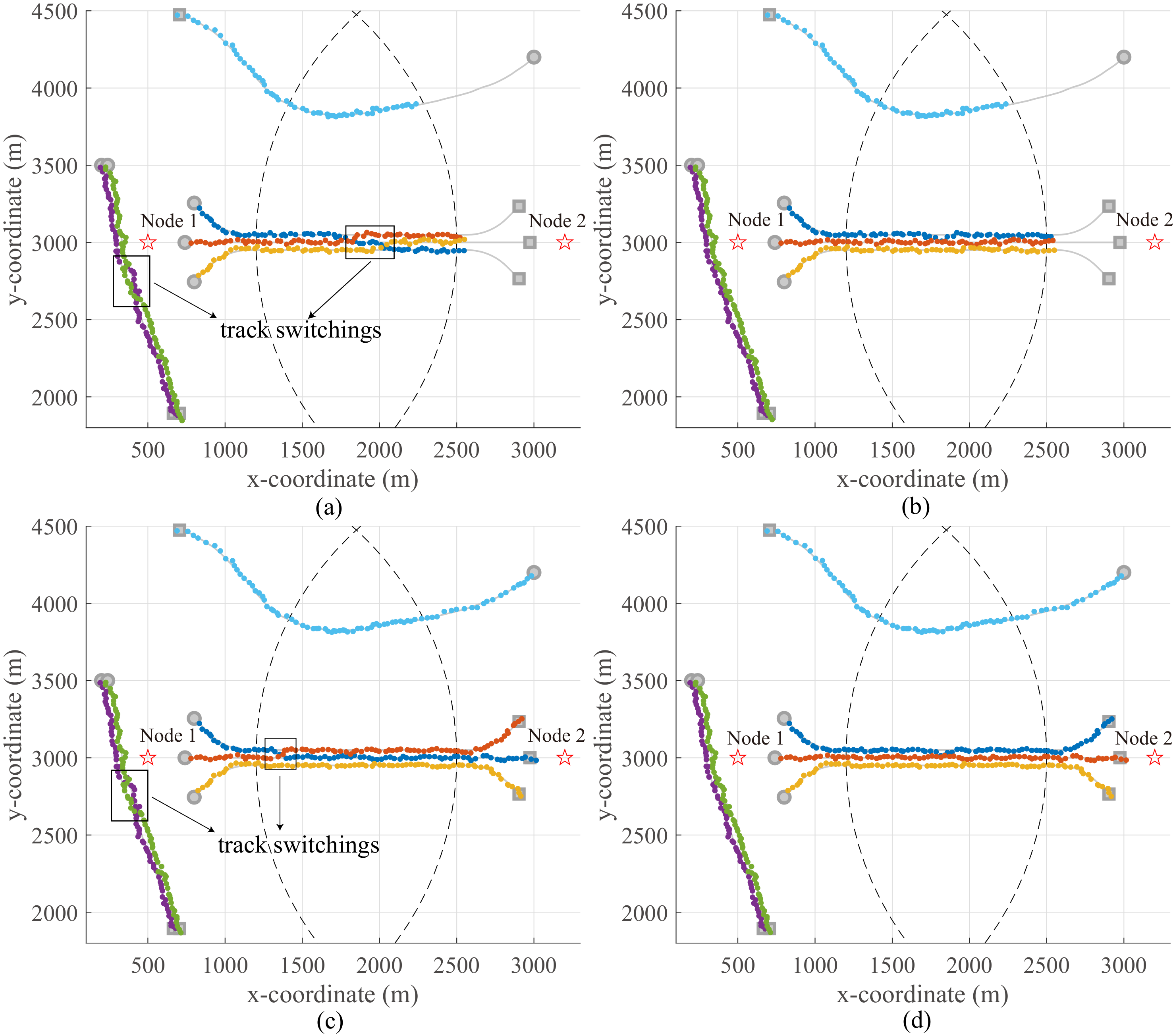
Figure 4 The estimated trajectories tracked by different methods at sensor 1 in scenario 1, where the color coding represents target identities. (a) BP; (b) GTBP; (c) DBP; (d) DGTBP.

Figure 5 The average tracking errors of all sensor nodes in scenario 1. (a) OSPA distance; (b) OSPA⁽²⁾ distance.

Figures 4(a)-4(d) plot the true trajectories and the estimated trajectories tracked by BP, GTBP, DBP, and DGTBP at sensor 1 of one example run, respectively. As shown in Figures 4(a)-4(b), BP and GTBP only can detect targets in the FoV of sensor 1 due to the limitation of FoV, and GTBP obtains better tracking performance (e.g., fewer track switchings) than BP for the reasons of jointly estimating the group structure uncertainty and enabling flexible modeling of group motions and single-target motions. Figures 4(c)-4(d) show that DBP and DGTBP can successfully detect and track all targets inside and outside the FoV of sensor 1 with the complement information from sensor 2, which significantly improve the tracking performance than BP and GTBP used for a single limited FoV sensor. Simultaneously, benefiting from the merits of GTBP for tracking group targets, DGTBP has fewer track switchings and can handle group splitting and merging more accurately than DBP, thereby obtaining better tracking accuracy, which is further verified in Figure 5.

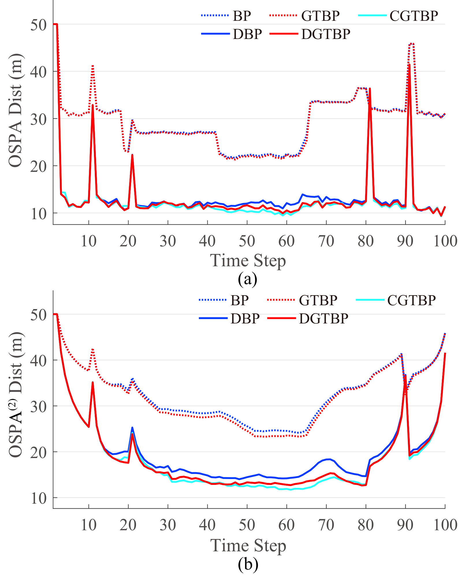
Figures 5(a)-5(b) plot the average OSPA and OSPA⁽²⁾ distances for scenario 1 over 50 MC runs versus the time step, where the spikes result from the track initiation, termination delays and window effects. The comparison results are consistent with the phenomena shown in Figure 4. More specifically, DGTBP and DBP overcome the limitation of FoVs and further reduce the tracking errors by making full use of the complementary information obtained from sensor 2, and DGTBP obtains better tracking accuracy than DBP. The reasons are the same as those analyzed for Figure 4. Furthermore, the performance of DGTBP is close to that of CGTBP.

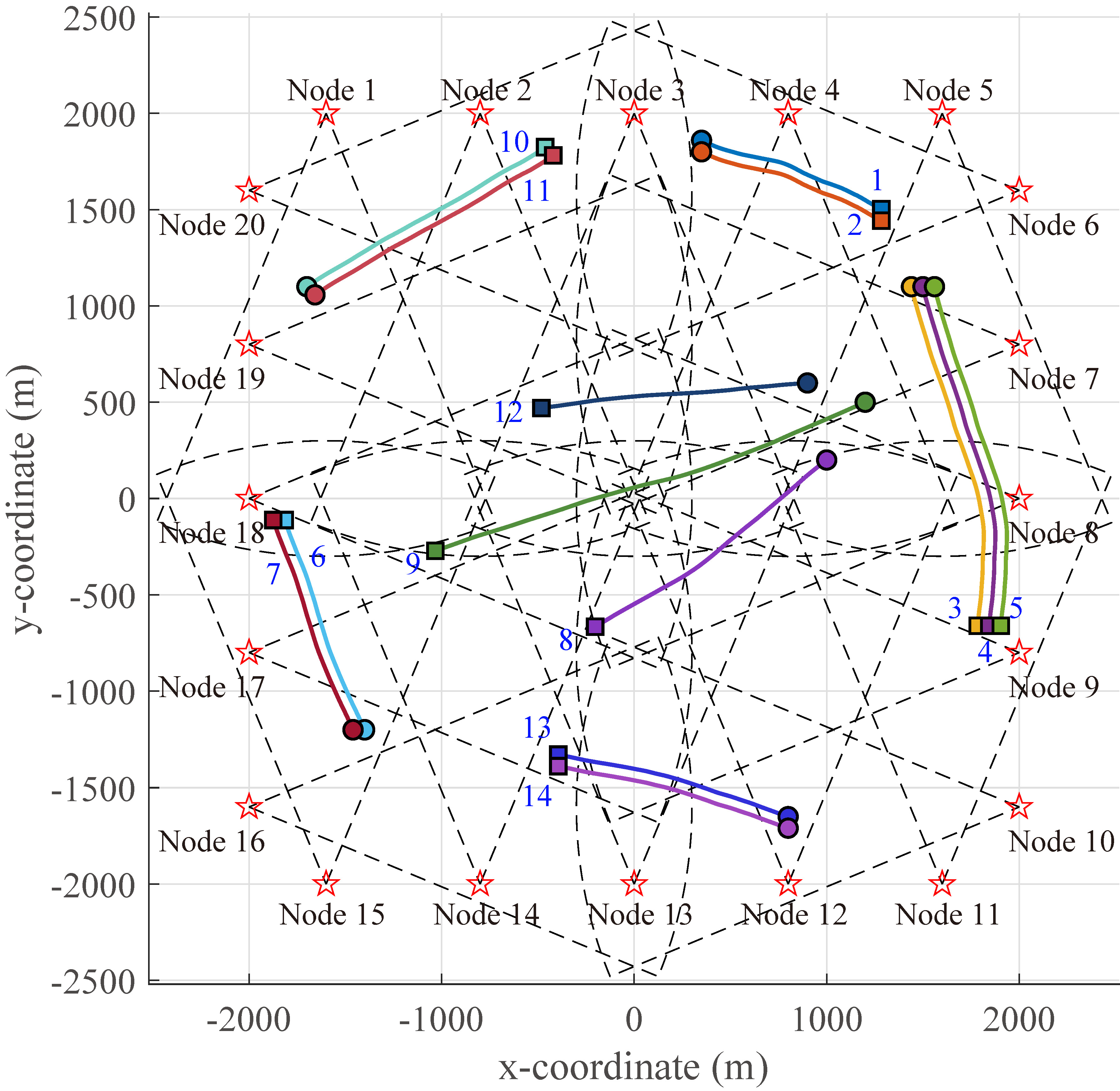
Next, we consider a more complex scenario with multi-sensor, multiple group targets and ungrouped targets. The simulated ground truths, sensor locations, and FoVs are shown in Figure 6. A total of 14 targets (including 5 group targets and 3 ungrouped targets) are simulated with various birth and death times. The maximum possible number of PTs is set to $27$ when using CGTBP, and otherwise $18$ . There are 5 sensors in the network, where sensors 1-4 have a limited FoV with a relative angle of interval $[-45^{\circ},\ 45^{\circ}]$ and a radius of 2100 m, and sensor 5 is with a relative angle of interval $[-180^{\circ},\ 180^{\circ}]$ and a radius of 1500 m. In this DSN, sensor 5 can exchange information with the other four sensors. The pruning length threshold is set to $K_{\mathrm{pr}}=3$ in the implementations of DBP and DGTBP.

Figure 6 The sensor nodes and ground truths simulated in scenario 2.

5.3 Scenario 2: Five Nodes with Multiple Group Targets and Ungrouped Targets

Figure 7 The estimated trajectories tracked by different methods at sensor 5 in scenario 2, where the color coding represents target identities. (a) BP; (b) GTBP; (c) DBP; (d) DGTBP.

Figure 8 The average tracking errors of sensor 5 in scenario 2. (a) OSPA distance; (b) OSPA⁽²⁾ distance.

Figures 7(a)-7(d) plot the true trajectories and the estimated trajectories tracked by BP, GTBP, DBP, and DGTBP at sensor 5 of one example run, respectively. On the whole, the comparison results shown in Figure 7 are similar those shown in Figure 4. Notably, DBP may further intensify the confusion on target identities when performing distributed information fusion for the targets within groups (that located in the overlapping FoV), leading to the performance degradation (see Figures 7(a) and 7(c)). Furthermore, DGTBP can successfully detect and seamlessly track all group targets and ungrouped targets inside or outside the FoV of sensor 5, which further demonstrate the effectiveness of DGTBP.

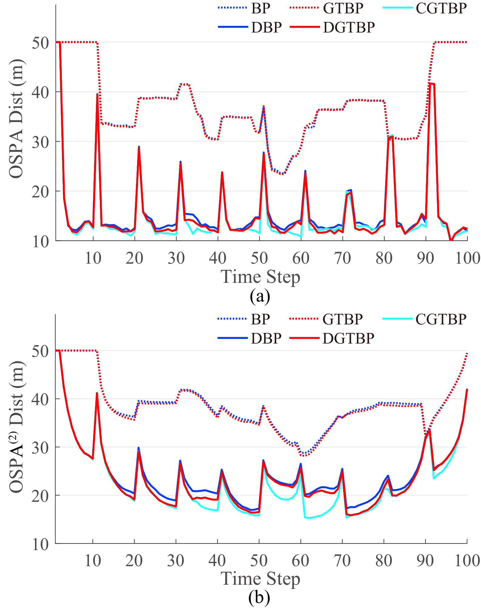
Figures 8(a)-8(b) plot the average OSPA and OSPA⁽²⁾ distances for scenario 2 over 50 MC runs versus the time step. The comparison results are consistent with the phenomena shown in Figure 7, which confirm that DGTBP outperforms DBP, BP, and GTBP in terms of the average OSPA and OSPA⁽²⁾. The reasons are the same as those analyzed for scenario 1. Moreover, the tracking performance of DGTBP is close to that of CGTBP.

5.4 Scenario 3: A Large-scale DSN

Figure 9 The sensor nodes and ground truths simulated in scenario 3.

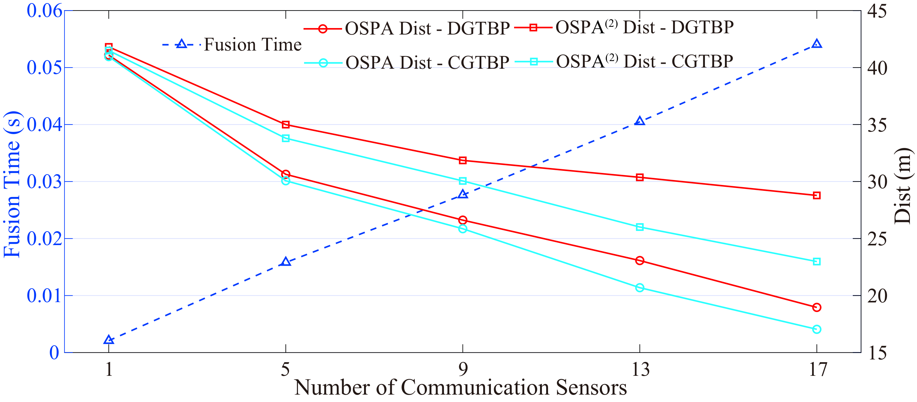
In scenario 3, we investigate how the fusion time scales in the network size to demonstrate the excellent scalability and low complexity of DGTBP. We simulate a DSN with 20 sensors for tracking 14 targets (including multiple groups and ungrouped targets) with different birth and death times, where the maximum possible number of PTs is set to $30$ when using CGTBP, and otherwise $20$ . The simulated ground truths, sensor locations, and FoVs are shown in Figure 9, where each sensor's FoV is with a relative angle of interval $[-22.5^{\circ},\ 22.5^{\circ}]$ and a radius of 2300 m. Due to higher uncertainty of this scenario, the pruning length threshold is set to $K_{\mathrm{pr}}=5$ in the implementations of DBP and DGTBP.

Figure 10 plots the average fusion time per consensus iteration, the average OSPA distance, and the average OSPA⁽²⁾ distance over 100 time steps and 10 MC runs versus the number of communication sensors at sensor 4 (i.e., the number of sensors exchanging information with sensor 4). The results indicate that the average fusion time per consensus iteration scales linearly in the number of neighboring sensors, which is consistent with the analysis in Section 3.4. Moreover, DGTBP inherits the same scalability as GTBP in the processing of local sensor data, i.e., scaling linearly in the numbers of preserved group partitions and local sensor measurements, and quadratically in the number of targets. Furthermore, with the increase of the number of communication sensors, the OSPA and OSPA⁽²⁾ errors decrease. The reason is that the use of multi-sensor allows for greater temporal and spatial coverage, and better precision (within the overlapping FoVs) than individual sensors with limited FoVs. As a consequence, DGTBP has excellent scalability and low complexity, which is applicable for the DGTT problem.

Figure 10 The average fusion time per consensus iteration, the average OSPA and OSPA⁽²⁾ distances at sensor 4 versus the number of its communication sensors.

6. Conclusion

This paper focuses on the DGTT problem under sensors with limited FoVs, and propose a scalable DGTBP method. By considering the group structure uncertainty, the proposed method can seamlessly track the group targets and ungrouped targets and accurately capture changes in group structure such as group splitting and merging. To deal with the target identity inconsistency of local sensors caused by different FoVs and distributed architecture, we efficiently solve the track association problem based on the BP scheme and perform the consensus fusion in a probabilistic way. Particularly, DGTBP has excellent scalability and low computational complexity that only scales linearly in the numbers of group partitions, local measurements, and neighboring sensors, and quadratically in the number of PTs. Numerical results for challenging DGTT scenarios demonstrate the effectiveness of DGTBP.

Data Availability Statement

Data will be made available on request.

Funding

This work was supported by the Natural Science Foundation of Sichuan Province under Grant 2025ZNSFSC0821 and the Special Fund for Postdoctoral Research Projects of Sichuan Province under Grant TB2024075.

Conflicts of Interest

The authors declare no conflicts of interest.

Ethical Approval and Consent to Participate

Not applicable.

References

Gadaleta, S., Poore, A. B., Roberts, S., & Slocumb, B. J. (2004, August). Multiple hypothesis clustering and multiple frame assignment tracking. In Signal and Data Processing of Small Targets 2004 (Vol. 5428, pp. 294-307). SPIE.
[CrossRef] [Google Scholar]
Mihaylova, L., Carmi, A. Y., Septier, F., Gning, A., Pang, S. K., & Godsill, S. (2014). Overview of Bayesian sequential Monte Carlo methods for group and extended object tracking. Digital Signal Processing, 25, 1-16.
[CrossRef] [Google Scholar]
Wang, Y., Shan, M., Yue, Y., & Wang, D. (2019). Vision-based flexible leader–follower formation tracking of multiple nonholonomic mobile robots in unknown obstacle environments. IEEE Transactions on Control Systems Technology, 28(3), 1025-1033.
[CrossRef] [Google Scholar]
Li, Q., Ahmad, B. I., & Godsill, S. J. (2021). Sequential dynamic leadership inference using Bayesian Monte Carlo methods. IEEE Transactions on Aerospace and Electronic Systems, 57(4), 2039-2052.
[CrossRef] [Google Scholar]
Mallick, M., Krishnamurthy, V., & Vo, B. N. (Eds.). (2012). Integrated tracking, classification, and sensor management: theory and applications. John Wiley & Sons.
[Google Scholar]
Zhu, Y. (2003). Multisensor Decision and Estimation Fusion. Kluwer Academic Publishers.
[Google Scholar]
Gning, A., Mihaylova, L., Maskell, S., Pang, S. K., & Godsill, S. (2010). Group object structure and state estimation with evolving networks and Monte Carlo methods. IEEE Transactions on Signal Processing, 59(4), 1383-1396.
[CrossRef] [Google Scholar]
Chong, C. Y. (1990). Distributed multitarget multisensor tracking. Multitarget-multisensor tracking: Advanced applications, 247-296.
[Google Scholar]
Battistelli, G., & Chisci, L. (2014). Kullback–Leibler average, consensus on probability densities, and distributed state estimation with guaranteed stability. Automatica, 50(3), 707-718.
[CrossRef] [Google Scholar]
Mahler, R. P. (2000, August). Optimal/robust distributed data fusion: a unified approach. In Signal Processing, Sensor Fusion, and Target Recognition IX (Vol. 4052, pp. 128-138). SPIE.
[CrossRef] [Google Scholar]
Hurley, M. B. (2002, July). An information theoretic justification for covariance intersection and its generalization. In Proceedings of the fifth international conference on Information Fusion. FUSION 2002.(IEEE Cat. No. 02EX5997) (Vol. 1, pp. 505-511). IEEE.
[CrossRef] [Google Scholar]
Julier, S. J., Bailey, T., & Uhlmann, J. K. (2006, September). Using exponential mixture models for suboptimal distributed data fusion. In 2006 IEEE Nonlinear Statistical Signal Processing Workshop (pp. 160-163). IEEE.
[CrossRef] [Google Scholar]
Ueney, M., Clark, D. E., & Julier, S. J. (2013). Distributed fusion of PHD filters via exponential mixture densities. IEEE Journal of Selected Topics in Signal Processing, 7(3), 521-531.
[CrossRef] [Google Scholar]
Li, T., Corchado, J. M., & Sun, S. (2018). Partial consensus and conservative fusion of Gaussian mixtures for distributed PHD fusion. IEEE Transactions on Aerospace and Electronic Systems, 55(5), 2150-2163.
[CrossRef] [Google Scholar]
Li, T., & Hlawatsch, F. (2021). A distributed particle-PHD filter using arithmetic-average fusion of Gaussian mixture parameters. Information Fusion, 73, 111-124.
[CrossRef] [Google Scholar]
Koliander, G., El-Laham, Y., Djurić, P. M., & Hlawatsch, F. (2022). Fusion of probability density functions. Proceedings of the IEEE, 110(4), 404-453.
[CrossRef] [Google Scholar]
Battistelli, G., Chisci, L., Fantacci, C., Farina, A., & Graziano, A. (2013). Consensus CPHD filter for distributed multitarget tracking. IEEE Journal of Selected Topics in Signal Processing, 7(3), 508-520.
[CrossRef] [Google Scholar]
Li, S., Battistelli, G., Chisci, L., Yi, W., Wang, B., & Kong, L. (2018). Computationally eff i cient multi-agent multi-object tracking with labeled random finite sets. IEEE Transactions on Signal Processing, 67(1), 260-275.
[CrossRef] [Google Scholar]
Üney, M., Houssineau, J., Delande, E., Julier, S. J., & Clark, D. E. (2019). Fusion of finite-set distributions: Pointwise consistency and global cardinality. IEEE Transactions on Aerospace and Electronic Systems, 55(6), 2759-2773.
[CrossRef] [Google Scholar]
Shen, K., Dong, P., Jing, Z., & Leung, H. (2021). Consensus-based labeled multi-Bernoulli filter for multitarget tracking in distributed sensor network. IEEE Transactions on Cybernetics, 52(12), 12722-12733.
[CrossRef] [Google Scholar]
Van Nguyen, H., Rezatofighi, H., Vo, B. N., & Ranasinghe, D. C. (2021). Distributed multi-object tracking under limited field of view sensors. IEEE Transactions on Signal Processing, 69, 5329-5344.
[CrossRef] [Google Scholar]
Kschischang, F. R., Frey, B. J., & Loeliger, H. A. (2002). Factor graphs and the sum-product algorithm. IEEE Transactions on information theory, 47(2), 498-519.
[CrossRef] [Google Scholar]
Meyer, F., Kropfreiter, T., Williams, J. L., Lau, R., Hlawatsch, F., Braca, P., & Win, M. Z. (2018). Message passing algorithms for scalable multitarget tracking. Proceedings of the IEEE, 106(2), 221-259.
[CrossRef] [Google Scholar]
Meyer, F., Braca, P., Willett, P., & Hlawatsch, F. (2017). A scalable algorithm for tracking an unknown number of targets using multiple sensors. IEEE Transactions on Signal Processing, 65(13), 3478-3493.
[CrossRef] [Google Scholar]
Soldi, G., Meyer, F., Braca, P., & Hlawatsch, F. (2019). Self-tuning algorithms for multisensor-multitarget tracking using belief propagation. IEEE Transactions on Signal Processing, 67(15), 3922-3937.
[CrossRef] [Google Scholar]
Sun, M., Davies, M. E., Proudler, I. K., & Hopgood, J. R. (2022). Adaptive kernel Kalman filter based belief propagation algorithm for maneuvering multi-target tracking. IEEE Signal Processing Letters, 29, 1452-1456.
[CrossRef] [Google Scholar]
Sharma, P., Saucan, A. A., Bucci, D. J., & Varshney, P. K. (2019). Decentralized Gaussian filters for cooperative self-localization and multi-target tracking. IEEE Transactions on Signal Processing, 67(22), 5896-5911.
[CrossRef] [Google Scholar]
Kropfreiter, T., & Hlawatsch, F. (2020, July). A probabilistic label association algorithm for distributed labeled multi-Bernoulli filtering. In 2020 IEEE 23rd International Conference on Information Fusion (FUSION) (pp. 1-8). IEEE.
[CrossRef] [Google Scholar]
Meyer, F., & Williams, J. L. (2020, May). Scalable detection and tracking of extended objects. In ICASSP 2020-2020 IEEE International Conference on Acoustics, Speech and Signal Processing (ICASSP) (pp. 8916-8920). IEEE.
[CrossRef] [Google Scholar]
Meyer, F., & Williams, J. L. (2021). Scalable detection and tracking of geometric extended objects. IEEE Transactions on Signal Processing, 69, 6283-6298.
[CrossRef] [Google Scholar]
Lau, R. A., & Williams, J. L. (2013, April). Tracking a coordinated group using expectation maximisation. In 2013 IEEE eighth international conference on intelligent sensors, sensor networks and information processing (pp. 282-287). IEEE.
[CrossRef] [Google Scholar]
Zhang, X., Liu, H., Zhong, J., & Shen, X. (2023). A scalable group target tracking method via belief propagation. Acta Aeronautica et Astronautica Sinica, 44(S2), 729761.
[Google Scholar]
Gordon, N. T., Salmond, D. J., & Fisher, D. J. (1997, October). Bayesian target tracking after group pattern distortion. In Signal and Data Processing of Small Targets 1997 (Vol. 3163, pp. 238-248). SPIE.
[CrossRef] [Google Scholar]
Mahler, R. P. S. (2007). Statistical Multisource-Multitarget Information Fusion. Artech House.
[Google Scholar]
Pang, S. K., Li, J., & Godsill, S. J. (2011). Detection and tracking of coordinated groups. IEEE Transactions on Aerospace and Electronic Systems, 47(1), 472-502.
[CrossRef] [Google Scholar]
Ristic, B., & Arulampalam, S. (2012). Bernoulli particle filter with observer control for bearings-only tracking in clutter. IEEE Transactions on Aerospace and Electronic systems, 48(3), 2405-2415.
[CrossRef] [Google Scholar]
Xiao, L., Boyd, S., & Lall, S. (2005, April). A scheme for robust distributed sensor fusion based on average consensus. In IPSN 2005. Fourth International Symposium on Information Processing in Sensor Networks, 2005. (pp. 63-70). IEEE.
[CrossRef] [Google Scholar]
Schuhmacher, D., Vo, B. T., & Vo, B. N. (2008). A consistent metric for performance evaluation of multi-object filters. IEEE transactions on signal processing, 56(8), 3447-3457.
[CrossRef] [Google Scholar]
Beard, M., Vo, B. T., & Vo, B. N. (2017, October). OSPA (2): Using the OSPA metric to evaluate multi-target tracking performance. In 2017 international conference on control, automation and information sciences (ICCAIS) (pp. 86-91). IEEE.
[CrossRef] [Google Scholar]

Cite This Article

APA Style

Liu, H., Zhang, X., Zhou, B., Liu, B., & Shen, X. (2025). Distributed Group Target Tracking under Limited Field-of-View Sensors Using Belief Propagation. Chinese Journal of Information Fusion, 2(3), 194–211. https://doi.org/10.62762/CJIF.2025.314716

Article Metrics

Citations:

Google Scholar

Crossref

Scopus

Web of Science

Article Access Statistics:

PDF Downloads: 14

Publisher's Note

ICCK stays neutral with regard to jurisdictional claims in published maps and institutional affiliations.

Rights and permissions

Copyright © 2025 by the Author(s). Published by Institute of Central Computation and Knowledge. This article is an open access article distributed under the terms and conditions of the Creative Commons Attribution (CC BY) license (https://creativecommons.org/licenses/by/4.0/), which permits use, sharing, adaptation, distribution and reproduction in any medium or format, as long as you give appropriate credit to the original author(s) and the source, provide a link to the Creative Commons licence, and indicate if changes were made.

Chinese Journal of Information Fusion

ISSN: 2998-3371 (Online) | ISSN: 2998-3363 (Print)

Email: [email protected]

Portico

All published articles are preserved here permanently:
https://www.portico.org/publishers/icck/