1. Introduction

Currently, with the deep and extensive popularization of high-precision sensors in cutting-edge fields such as autonomous driving, robot navigation, and security monitoring, extended target tracking (ETT) technology has emerged as a new research hotspot [1, 2]. Compared to the issue of traditional point target tracking, extended target tracking encompasses multiple information dimensions such as position, shape and velocity, which undoubtedly poses more stringent requirements on the accuracy and complexity of tracking algorithms [3].

(a) Simulation scene

(b) Sensor distribution

(c) Tracking results

Figure 1 An autonomous driving scenario: A car with radar and vision sensors is driving on a highway.Due to the presence of occlusion, the truck is mistakenly recognized as two targets, resulting in a split situation.

To achieve effective tracking of extended targets, numerical methods have been addressed. For example, Granstrom et al. [4] introduced probability hypothesis density (PHD) filter and cardinalized probability hypothesis density (CPHD) filter into the ETT field. Then two measurement set partitioning methods [5] were added into the filters in [4]. Additionally, Habtemariam et al. [6] integrated the measurement unit generation strategy with joint probability data association (JPDA), thereby proposed the multi-detection joint probability data association (MD-JPDA) method. Zhang et al. [7] introduced the cardinality balanced multi-target multi-Bernoulli (CBMeMBer) algorithm and successfully conducted the ETT task. In [8], the generalized labeled multi-Bernoulli (GLMB) and Gamma Gaussian inverse Wishart (GGIW) distributions were used to precisely model the states and extension characteristics of multiple extended targets. Then, the GGIW Poisson model was ingeniously embedded into the multi-Bernoulli filter to cope with the issue of multi-extended target tracking [9]. Recently, an approach based on irregular probability distributions has also been proposed to cope with this issue [10].

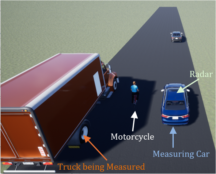
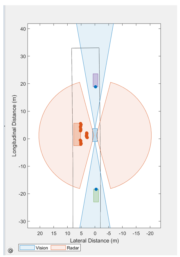
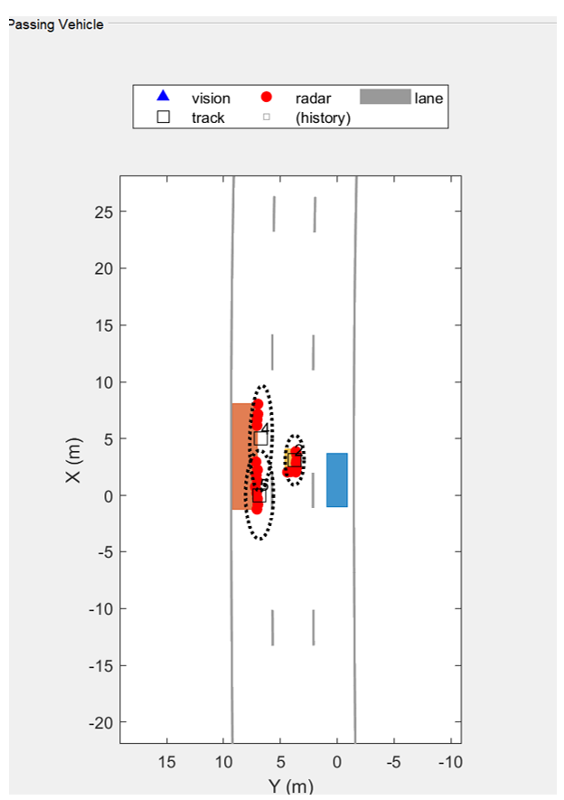
However, when extended targets are occluded or densely distributed, due to their non-point nature and their complex interaction patterns in dynamic environments, the methods mentioned above are prone to trigger the challenging problem of target splitting or merging during actual operation. For example, in Figure 1(a), the radar of the car is occluded by a motorcycle, resulting in the truck being identified as two split targets, as shown in Figure 1(c). To cope with this problem, the key lies in accurately distinguishing whether the target has truly split or it is merely false alarm.

A few related works have been proposed to address the above problem. For visual targets, [11] detected target splitting positions and segments trajectories by stacking temporal dilated convolution blocks and an adaptive Gaussian smoothing label strategy. For missile targets, [12] constructed a mathematical model for splitting event detection and tracking within the joint integrated probabilistic data association (JIPDA) framework, achieving point target splitting determination and tracking through probability calculations of splitting events. [13] optimized the de-correlation time of group targets using Pareto analysis based on the interactive multiple model-unscented Kalman filter (IMM-UKF) framework, which essentially performs data association on point targets within group targets. It is important to note that these methods only utilize the position data of point targets. Directly applying them in extended target tracking scenarios cannot fully leverage the extended information of targets, leading to poor performance. To the best of our knowledge, there has been no work addressing the problem of splitting and merging of extended targets so far.

Motivated by this, we aim to make use of extended information and achieve accurate determination and fusion of split targets. To this end, we first analyze the extended target splitting problem with PHD-based filters, and then present the similarity of the track feature of extended targets. Next, we expand spatio-temporal [14] based clue-aware trajectory similarity (CATS) method to the ETT issue by integrating the Gaussian Wasserstein (GW) distance. Subsequently, we develop an extended target split error correction algorithm.

In summary, the main contribution of this paper is the proposed method that can solve the splitting problem of extended targets by using the spatio-temporal trajectories and extended information of extended targets. Furthermore, as far as we know, the method presented in this paper is the first work to deal with the issue of the split of extended target.

The organization of this paper is as follows. Section 2 describes the problem of extended target splitting in detail. Section 3 analyzes the split tracks' information. Section 4 elaborates on the proposed splitting determination method. Section 5 builds a simulation scenario to verify the effectiveness of proposed method. Section 6 summarizes the entire paper.

2. Problem Formulation

3. Similarity Analysis of Track Feature

First of all, we will analyze the track feature of the split extended targets in this section.

As described above, an elliptic extended target information includes position $p$, detection time $t$ and geometric information $X$. This elliptic can be interpreted as the following Gaussian distribution [17]:

where ${𝐞}_{𝐠}$ is scaling factor relates to the tolerance region that is user-defined. In addition, due to the uncertainty of sensor measurement and data processing, the detection time can also be considered to obey the following Gaussian distribution:

where $△t$ is time interval and ${𝐞}_{𝐭}$ represents the scaling factor.

Suppose that track $T^{\cdot }$ which has already existed moves in a two-dimensional plane, after being tracked by the PHD-based filter, it splits into two tracks $T^i$ and $T^j$ with distribution sets $(ℰ{𝒯}^i,𝒩{𝒯}^i)$ and $(ℰ{𝒯}^j,𝒩{𝒯}^j)$, then their center sets $(p^i,t^i)$ and $(p^j,t^j)$ can be separately connected as a curve in a three-dimensional plane, as shown in Figure 2.

Figure 2 An illustration of spatio-temporal prism structure.

It can be observed that, influenced by various factors, there are deviations in the area where the two distributions should overlap, and the deviation shows the following characteristics: The deviations in detection time are highly random, but the deviations in spatial position are relatively fixed, and there are slight deviations in the rotation angle. Additionally, some measurement data are missing. Hence, if the two tracks are originated from the same track, they are actually a kind of spatio-temporal prism structure [18] with a range of uncertainty. Thus, we can use the similarity of historical track information to determine the split possibility of extended target.

In order to determine the split possibility, the clue-aware trajectory similarity (CATS) method based on spatial and temporal information in [19] is chosen. Its main idea is to find potential "matching points" on the two tracks when evaluating the spatial and temporal similarity. However, since it is inappropriate to use the center point to represent the extent of an ellipse, the direct application of the CATS method will result in unsatisfactory outcomes. Therefore, we propose a new method called GW-CATS to determine the splitting of extended targets, which will be elaborated in the next Section.

4. Extended Target Splitting Determination Method

Before introducing the determination method, we first introduce Gaussian Wasserstein distance [17].

For elements $T_a^i\in T^i$ and $T_b^j\in T^j$ , they can construct two elliptical extended targets subjected to the following Gaussian distributions:

The Gaussian Wasserstein distance between the two extended targets provides the similarity measure metric that is defined as:

where $Tr(\cdot )$ represents the trace operator.

This metric simultaneously captures positional offsets and quantifies the congruence between the two targets' shapes through their covariance matrices. In this article, $d_{GW}(ℰ{𝒯}_a^i,ℰ{𝒯}_b^j)$ will be represented by the shorthand notation $d_{GW}(T_a^i,T_b^j)$.

The main idea of the CATS method is to evaluate the spatial and temporal similarity of different tracks. The core workflow is as follows: First, temporal and spatial thresholds are set to filter elements contained in the two tracks, selecting element pairs from different tracks that are temporally and spatially close. Subsequently, the spatial distances between these element pairs are normalized to identify the most similar pairs. Lastly, the similarity between two tracks is computed as the average of all normalized similarity scores of their best-matching element pairs.

Since CATS handles point targets through Euclidean distance, it fails to account for extended target. Thus, we propose the GW-CATS method that addresses this limitation by incorporating geometric information, enabling a more reasonable use of extended information. The detailed implementation of the proposed method is as follows.

At time step $k$, suppose that the track information is obtained from the front-end tracker. Thereinto, $T^j$ represents a newborn track and $T^i$ represents an existing track. In order to calculate the similarity between track $T^i$ and track $T^j$, the following four-step process is adopted as follows:

Step 1: Spatio-temporal Matching Elements Finding

Given a spatial threshold $ϵ$, a time threshold $\tau$, two elements $T_b^j\in T^j$ and $T_a^i\in T^i$, if $T_b^j$ and $T_a^i$ satisfy the following conditions:

(1) $\left|t_b^j-t_a^i\right|\le \tau$, (2) $d_{GW}(T_b^j,T_a^i)\le ϵ$,

then we call $T_a^i$ is the spatio-temporal matching element of $T_b^j$ and $\left\{T_a^i\to T_b^j\right\}$ is a spatio-temporal matching pair.

Similar to the CATS method, we set a time threshold $ϵ$ and a space threshold $\tau$ to compensate for the uncertainty of target kinematics and sensor measurements. Due to the existence of extended target velocity information, After the determination of user-defined time threshold $ϵ$ according to the actual situation, the spatial threshold $\tau$ can be calculated by the following method.

Figure 3 Geometric illustration of the spatial threshold.

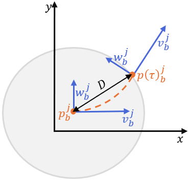
As shown in Figure 3, the initial center position of extended target $T_b^j$ is set as $p_b^j$, its speed is $v_b^j$, and turning rate perpendicular to the direction of the velocity vector is $w_b^j$. After passing time $\tau$, the center of the target $T{\left(\tau \right)}_b^j$ reaches the position $p{\left(\tau \right)}_b^j$. Since $\tau$ is relatively small, the target speed can be approximated as constant during the motion. Then, the Euclidean distance $D$ between point $p_b^j$ and $p{\left(\tau \right)}_b^j$ can be expressed as:

where $\left|\right|\cdot |{|}_2$ denotes the 2-norm operator. Using $D$ as the radius, a validation gate is constructed to filter spatially irrelevant elements, as shown in gray part in Figure 3. Since $\tau$ is relatively small, the elliptical rotation angle $\alpha =w\tau$ remains minimal. By neglecting rotational effects, we derive:

The detailed derivation is provided in Appendix.

Step 2: Similarity Calculation of Matching Elements

For any elements in the reference track, the number of matching elements from other tracks may be zero, one, or multiple.

To distinguish matching elements and find the most similar matching pair, we quantify similarity scores through numerical normalization to the range [0,1], enabling optimal matching selection. Thus, the similarity of matching elements are calculated as follows [20] :

where $T_a^i$ is a matching element of $T_b^j$ and the value range of the function $f_{ϵ}\left(T_a^i\to T_b^j\right)$ is limited in [0,1]. The closer the position and geometric information of two ellipses are, the larger this function value is, indicating greater similarity. If two extended targets are exactly the same, this function's value equals to 1. For brevity, $f_{ϵ}\left(T_a^i\to T_b^j\right)$ will be abbreviated to $f^{ai\to bj}$.

Step 3: Best Matching Element Confirm

After similarity calculation, we can confirm the best matching element of $T_b^j$. Suppose that track $T^i$ contains $n$ elements, for $T_a^i\in T^i$, if:

then we call $T_a^i$ the best matching element of $T_b^j$, where $T_q^i$ represents any matching element of $T_b^j$ in track $T^i$.

Best matching element pairs are defined as those that optimally capture the same kinematic characteristics. When two tracks are hypothesized to originate from the same physical target, our objective is to systematically identify these optimal element pairs, thereby enabling the subsequent processing step.

Step 4: Similarity Calculate of Two Tracks

Finally, after the above three steps, we obtain the best matching elements and matching values of each elements in track $T^j$. The inter-track similarity is determined by aggregating and averaging the normalized similarity scores across all matched element pairs. Thus, the spatio-temporal similarity of track $T^i$ to track $T^j$ is defined as:

where $\left|T^j\right|$ refers to the number of elements in $T^j$ and $T_a^i$ is the corresponding best matching element of $T_b^j$. For brevity, $S_{ϵ,\tau }\left(T^i\to T^j\right)$ will be abbreviated to $S^{i\to j}$. In summary, a complete pseudocode implementation of the proposed method is provided in Algorithm 1.

For any newborn track $T^j$, its similarity score $S^{i\to j}$ with respect to each established independent track $T^i$ can be systematically computed through Algorithm 1. By establishing a similarity threshold $\mu$, we implement the following decision rule:

If two tracks are determined to be similar, the Monte Carlo Minimum Mean Gaussian Wasserstein (MC-MMGW) method can be used to fuse the information of the two extended targets. For the specific details of the fusion method, please refer to reference [21].

5. Numerical Experiments

In this section, we set a highway autonomous driving simulation scenario to evaluate the proposed GW-CATS method. We used the optimal sub-pattern assignment (OSPA) [22] and generalized optimal sub-pattern assignment (GOSPA) [23] as evaluation metric to Verify the effectiveness of the proposed GW-CATS method.

5.1 Simulation Scene Settings

Given $k=136$ time steps, $t=13.6s$ in total, we first set up the simulation scenario. The scenario is set in two-dimensional three-lane highway with lane width 3.5 m. The road centerline coordinates is [0 0 ; 50 0 ; 100 0 ; 250 20 ; 400 35]m. There are a total of five vehicles on the highway, and they all travel along the corresponding lane. Target parameters are listed in Table 1.

Table 1 Target parameters.

Parameter	Dimensions	Velocity	Lifetime
	(m2)	(m/s)	(s)
RadarCar	4.7$\times$1.8	$25-\frac{t}{20}$	0.1-13.6
Target 1	4.7$\times$1.8	25	0.1-13.6
Target 2	2.0$\times$1.0	24	0.2-13.6
Target 3	4.7$\times$1.8	26	0.3-13.6
Target 4	9.3$\times$2.2	$35-\frac{t^2}{142}$	0.1-13.6

Specifically, target 4 represents a motorcycle, target 1 is a truck, Target 2 and 3 are standard vehicles. The RadarCar is an autonomous vehicle equipped with four radars, and radar parameters are listed below:

(a) Tracking results of the GGIW-PHD filter.

(b) Tracking results of the GGIW-PHD filter corrected by GW-CATS method correction.

Figure 4 Tracking results in single run simulation scenario.

• Left/Right radars: 160° detection angle, 30 m range.

• Front/rear radars: 30° detection angle, 50 m range.

• Detection probability $P_d=0.9$.

• False alarm rate ${\lambda }_{fa}=1\times {10}^{-6}$.

• Clutter intensity ${\lambda }_{ck}=8$ (Poisson point process distribution).

The GGIW-PHD filter is used to track these targets, its corresponding parameters are shown in Table 2. For the specific introduction of the parameters, please refer to [16].

Table 2 GGIW-PHD filter parameters.

Parameter	Value
Birth rate	$1\times {10}^{-3}$
Death rate	$1\times {10}^{-6}$
Assignment threshold	220
Extraction threshold	0.8
Confirmation threshold	0.95
Deletion threshold	$1\times {10}^{-3}$
Labeling threshold	[1.1 1 0.8]
Merging threshold	50

5.2 Experimental Results

A.Selection of Time Threshold

The selection of time threshold is a process that combines experience and mathematical principles. In GW-CATS method, the physical meaning of the time threshold $\tau$ is the maximum acceptable time interval between the split target and the original target, and its value is based on the theory of spatio-temporal trajectory similarity: if two trajectories originate from the same target split, their spatio-temporal distribution should maintain continuity in finite time.

Taking the simulation scenario in this section as an example, the speed of the split truck is $25m/s$ and its length is $10m$, then the time required for the target to completely cross its own length is $10÷25=0.4s$. Considering the geometric uncertainty of the elliptical target after splitting, $\tau =0.5s$ is finally selected as the equilibrium value. In order to verify the rationality of the threshold, a comparative experiment of $\tau \in [0.1,1.5]s$ is designed, and the key parameters are set as follows:

• Similarity threshold $\mu =0.7$.

• Time threshold $\tau =0.1-1.5s$.

• Newborn target validation step $k_{sim}=4$.

Figure 5 Sensitivity analysis of time threshold for GGIW-PHD filter corrected by GW-CATS method.

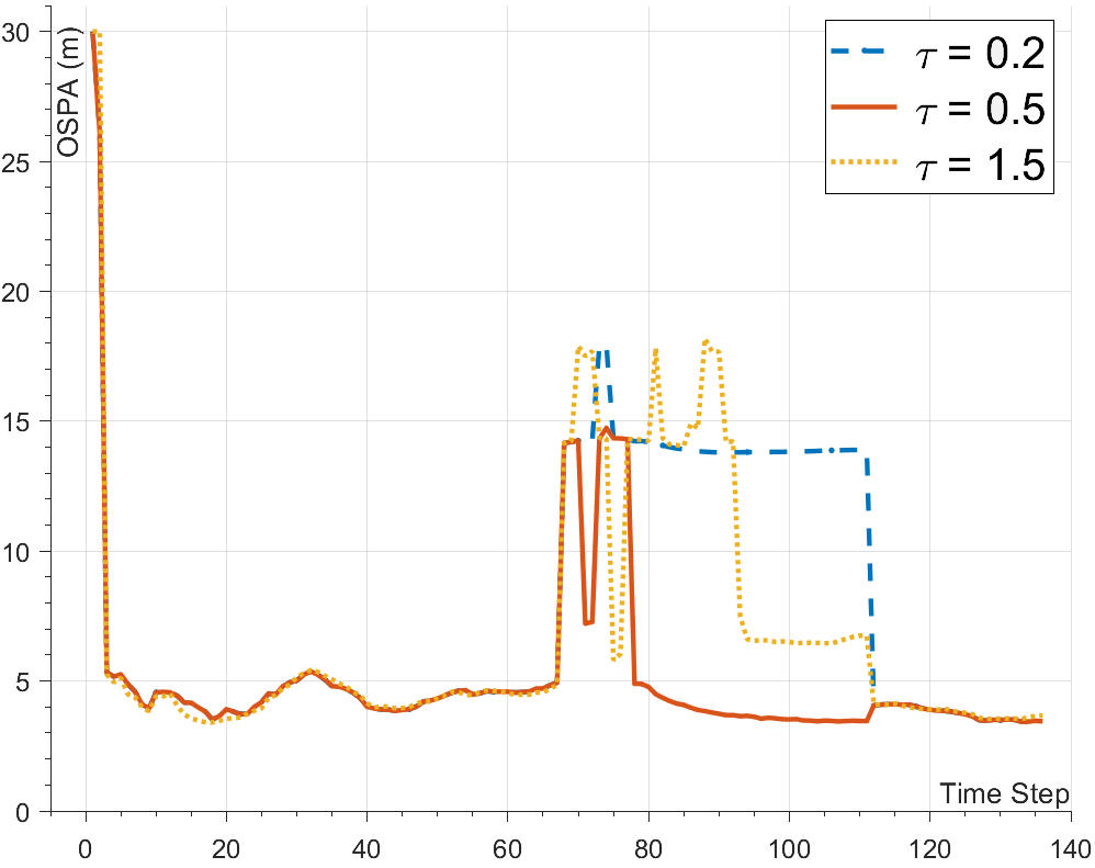
The experiments show that the tracking performance is optimal when $\tau \in [0.4,0.7]s$. When , the real split targets cannot be merged due to the excessively narrow time window, and when $\tau >0.7s$, adjacent targets are prone to false merging. Under different $\tau$ value, the OSPA metric are shown in Figure 5. In what follows, $\tau$ of the proposed GW-CATS method is uniformly taken as $0.5s$.

B. Single-Run Results

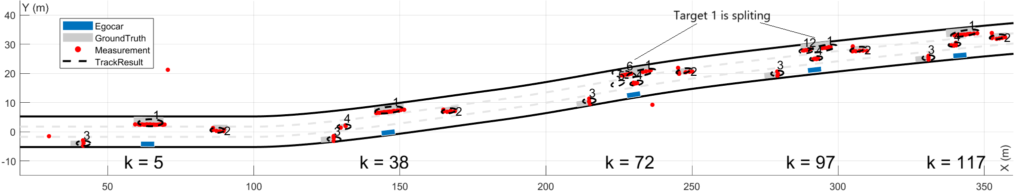
Figure 4(a) shows the GGIW-PHD tracking results. The detected targets are all represented in the form of elliptical extended targets. It is evident that for target 1 (truck), a distinct segmentation issue occurs after it is obstructed by target 4 (motorcycle), resulting in few false newborn track (target 5-12).

Figure 6 Fusion results. An inner tangent ellipse with the length and width of the rectangle as axes is used to represent the ground truth.

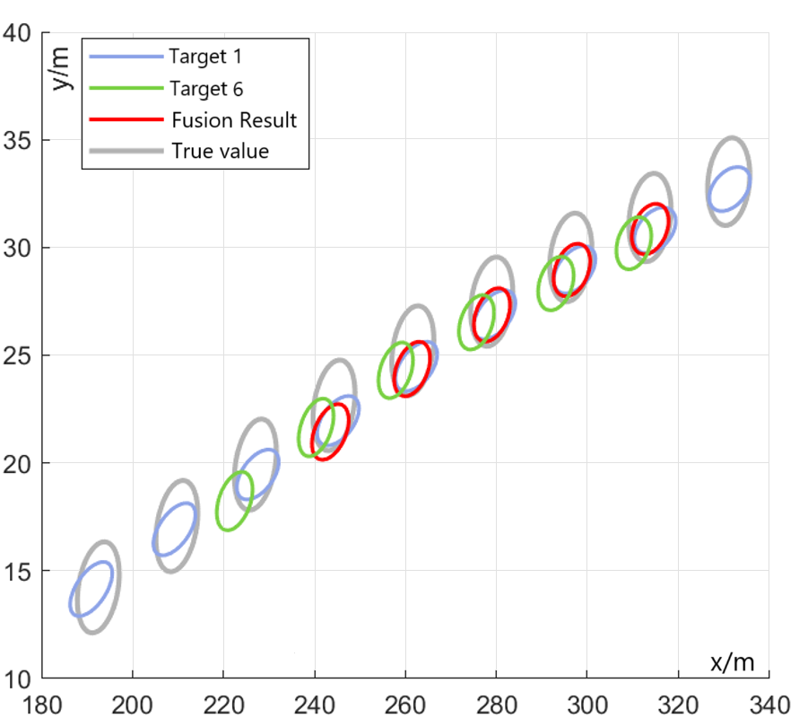
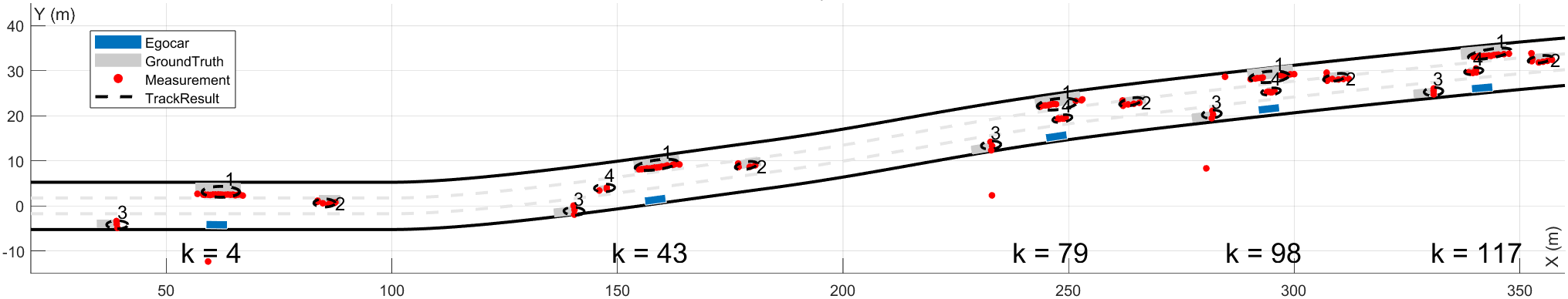
As comparison, Figure 4(b) shows the result with the proposed GW-CATS method. From $k=71$ to $k=79$, the truck target split into several false targets. Some of these false targets disappeared during their movement, while others remained until $k=117$. Taking target 6 generated at k = 72 as an example, after $k_{sim}$ iterations, at $k=75$, the similarity between new track 6 and tracks 1-4 is [0.845, 0.629, 0, 0.627], so the proposed GW-CATS method decided to fuse target 6 and 1. Further, at $k=97$ and $k=117$, the similarity between track 6 and track 1 is 0.896 and 0.910, respectively, so the target fusion process continued, and ultimately the proposed GW-CATS method successfully completed the split determination task. Futhermore, the fusion result is shown in Figure 6.

C.Monte Carlo Results

Figure 7 OSPA metric over 50 MC trails, [*] represents the GGIW-PHD Tracker.

Figure 8 GOSPA metric over 50 MC trails, [*] represents the GGIW-PHD Tracker.

To evaluate the performance of the GW-CATS method, this section introduces the point-target based CATS method and the global nearest neighbor (GNN) method for comparison with the proposed GW-CATS method. The parameters of the GW-CATS method are consistent with those described in 5.1. The specific parameters of the CATS method are as follows:

• Spatial threshold $ϵ=10m$.

• Time threshold $\tau =0.5s$.

The key parameter configurations of the GNN method are as follows:

• Assignment threshold = 30.

• Detect/Miss Confirmation threshold = [4/5].

• Deletion threshold = 3.

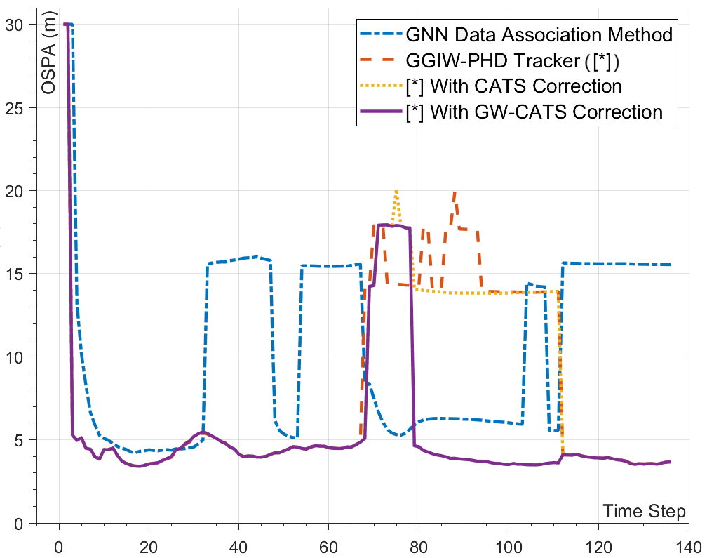
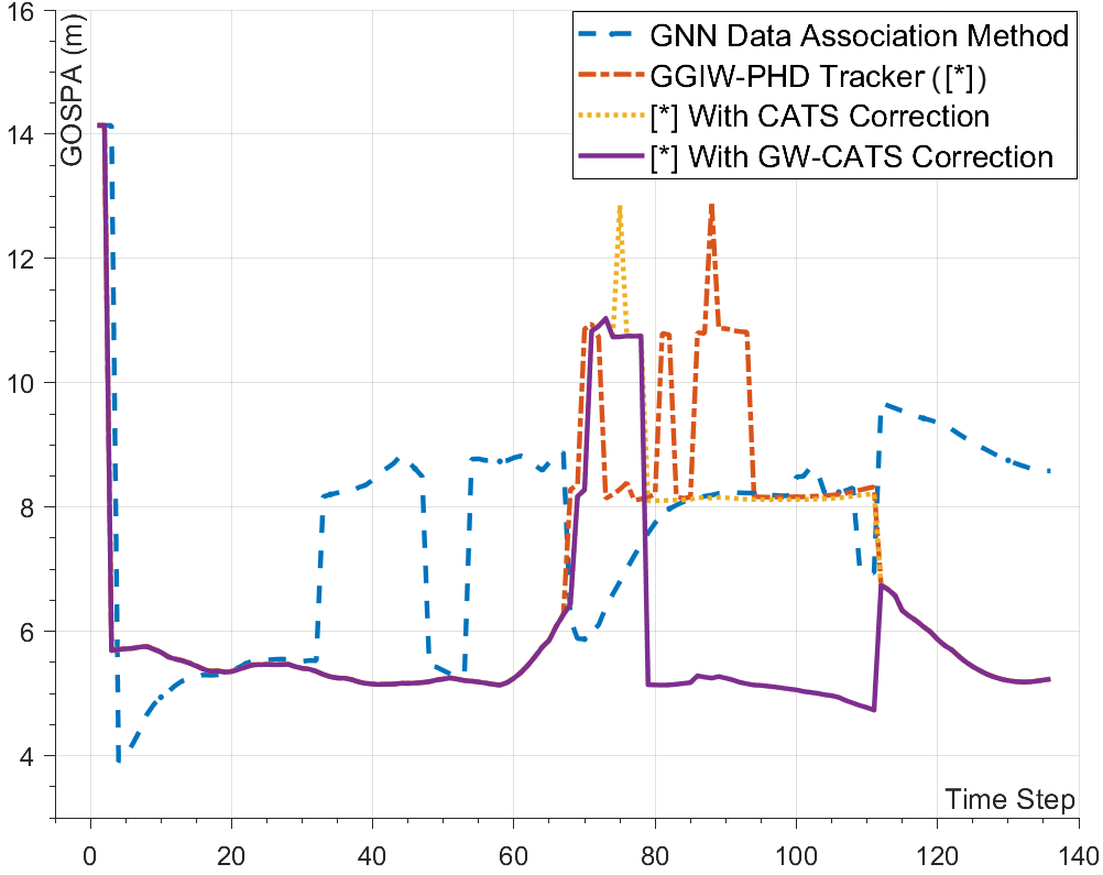
We futher conducted 50 Monte Carlo (MC) trails to demonstrate the effectiveness of the proposed GW-CATS method. The tracking error evaluated by the mean OSPA metric are shown in Figure 7. The tracking error evaluated by the mean GOSPA metric with $p=1$ and $c=10m$ are shown in Figure 8.

It can be observed that the OSPA or GOSPA value of the GGIW-PHD filter with GW-CATS correction is greatly reduced when the split target is successfully determined, compared with that of the original GGIW-PHD filter, GNN method and CATS method. It proves that the GW-CATS method can significantly improve the tracking accuracy of extended targets in occlusion scenes.

6. Conclusion

To address the splitting correction problem in extended target tracking under occlusion scenarios, we propose a novel track spliting determination method named GW-CATS that integrates the GW distance with spatio-temporal similarity analysis. Simulation results demonstrate that the proposed method can successfully determine the case of target splitting, further reduces the OSPA metric in split scenarios and achieves stable track fusion.

Appendix : The deviation of equation (3)

First, let us set time threshold $\tau$, $p_b^j=(x_0,y_0)$, $p{\left(\tau \right)}_b^j=(x_{\tau },y_{\tau })$, $v_b^j=(v_x,v_y)$ and turn-rate $w_b^j$. Then, the direction angle of the velocity vector at the initial time is $\alpha =\arctan \left(\frac{v_y}{v_x}\right)$, the angle of the target's rotation around the center of the circle is $\theta ={\omega }_b^j\tau$ and the radius of the arc is $r=\frac{{\Vert v_b^j\Vert }_2}{\left|w_b^j\right|}$. On the one hand, when $w_b^j\ne 0$, it follows that

Then, the Euclidean distance $D$ can be calculated by the following formula

Furthermore, on the other hand, when $w_b^j=0$, the velocity displacement formula can be directly applied for the calculation. Hence, it follows that: