





Abstract
Graphical Abstract
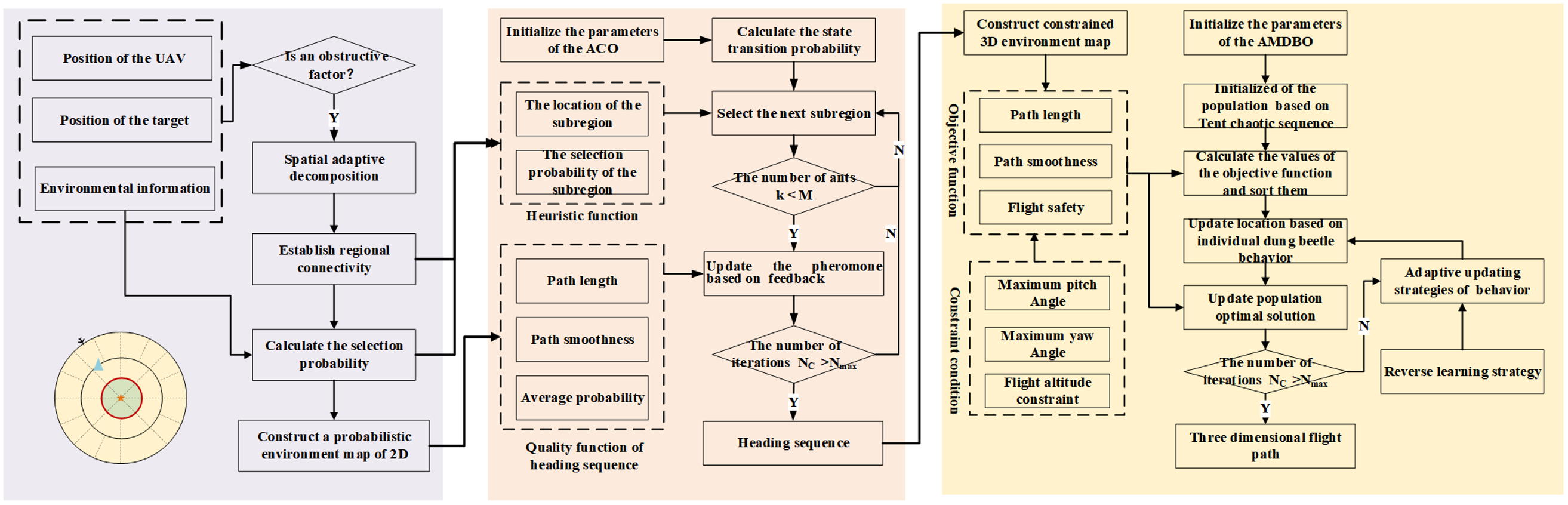
Click image to view fullscreen
Keywords
1. Introduction
With high maneuverability, strong concealment abilities, and resistance to interference, the UAV has emerged as a critical military tool for performing diverse tasks such as reconnaissance, airstrikes, and electronic warfare [1]. Effective path planning based on macro environmental information is pivotal in strategizing air defense force deployments and seizing tactical advantages [2]. Confronted with challenges from extensive airspace and complex environments leading to inefficient and suboptimal trajectory planning [3], efficient path planning has become a pressing technological need to address.
Path planning can be divided into global path planning, local path planning, and mixed path planning. Global path planning aims to apply planning algorithms to find a collision-free, safe, and short path from the starting point to the endpoint for the UAV within the constraints of the known environment [4]. This paper focuses on the comprehensive impact of a complex environment on mission performance and flight safety, which belongs to the scope of global path planning. Currently, existing global path planning algorithms can be roughly categorized into four groups: algorithms based on graph theory, fluid/potential field algorithms, swarm intelligence algorithms, and neural network methods. Graph theory methods mainly include the Dijkstra algorithm [5, 6], the A* algorithm [7, 8], and fast search random tree algorithm (RRT*) [9, 10]. Graph search is the most effective direct search method for solving the shortest path in a static road network. However, as the graph expands and dimensions increase, computational efficiency decreases rapidly. Fluid/potential field algorithms, such as artificial potential field [11, 12] and Interfered Fluid Dynamical System (IFDS) [13, 14] can generate a smooth virtual field based on the position of UAVs and obstacle distribution. These algorithms offer clear advantages in smooth path planning control and are widely applied. Swarm intelligence algorithms are self-organizing, adaptive, and self-learning. They can effectively solve UAV path planning, such as the Gray Wolf algorithm [15], Sand Cat algorithm [16], Particle Swarm Optimization algorithm [17], and Dung Beetle Optimization (DBO) [18]. Because of the heuristic search and positive feedback of information, Ant Colony Optimization (ACO) is more suitable for solving simple graph path search problems [19]. DBO is extensively used in 3D path planning due to its robust global search capability [20, 21, 22]. Neural networks possess strong nonlinear learning abilities and demonstrate good path-planning capabilities in complex environments [23, 24, 25]. In Reference [23], residual convolutional neural networks were used to solve the real-time path planning problem. Literature [24] proposed an improved TD3 algorithm to train UAVs to reach targets safely and quickly in multi-obstacle environments. However, the performance of neural networks heavily relies on adequate data and appropriate training, particularly in complex path-planning tasks that demand substantial computational resources. Moreover, in unfamiliar environments, neural networks may have limited generalization abilities require necessitate additional retraining to adapt to new environments.
The vast area increases the solution space for path planning, making it challenging to balance path exploration and convergence. The quality of the path is not guaranteed, and planning times are extended. Furthermore, in the military environment, focusing solely on the flight safety of UAVs is insufficient. Environmental factors such as terrain, visibility, and wind speed significantly impact the effectiveness of reconnaissance and penetration missions. To enhance operational efficiency and path safety, three crucial questions are identified for path planning in aerial environments: "Where can I go?" "Where should I go?" and "How should I get there?" [26]. Inspired by the divide-and-conquer concept, a new two-layer path planning method is proposed. Firstly, considering the influence of multi-dimensional environmental information on path planning, an adaptive 2D probabilistic map construction method is proposed to answer the question of "where to go". Secondly, an improved ant colony algorithm is proposed to guide UAVs in course sequence planning in 2D maps, and a series of sub-regions with high heading selection probability are obtained, which answers the question "where should go". Finally, the distribution information of obstacles in the heading area is analyzed, and the path optimization model is designed according to the maneuvering constraints of UAVs, which realizes the accurate trajectory optimization in 3D space and answers the question of "how to get there". The proposed two-layer path planning model focuses on different information in distinct layers, enhancing the efficiency and quality of path planning.
The main contributions of the paper are as follows. (1) Based on the divide and conquer concept, traditional path planning is segmented into heading planning and path optimization. The 3D path planning is carried out under the spatial constraints of the global heading planning results, which reduces the search space, ensuring the efficiency and quality of path planning. (2) A heading sequence planning model in large airspace is designed. An adaptive two-dimensional probabilistic map construction method based on multi-dimensional environment information is proposed, and the ant colony algorithm is improved to achieve efficient course planning in large airspace. (3) A trajectory optimization model in local airspace is designed. A multi-strategy Dung Beetle algorithm is proposed to enhance the efficiency and quality of path optimization in 3D space.
The remainder of this paper is organized as follows. Section 2 briefly introduces the relevant theories; Section 3 introduces the method proposed in this paper. Section 4 shows the simulation experiments and discussion. Section 5 presents the conclusions of this study.
2. Related Work
2.1 Ant colony optimization
Ant colony optimization (ACO) [27] is a bionic algorithm according to the law of the overall foraging behavior of the ant colony: the individuals in the ant colony will leave a chemical substance called "pheromone" on the walking path, and update the pheromone on each path as shown in Eq.(1):
where is the global pheromone volatilization coefficient. is the positive change of the pheromone on the path in the current iteration, as shown in Eq.(2).
where is the concentration of left pheromones by ant on path . If ant has not passed the path , the value is 0.
Other ant colonies will calculate the node transition probability based on Eq.(3) when making route selection.
where is the heuristic information, represents the degree of transition expectation of ant from node to node , is the pheromone concentration factor, is the expected heuristic factor. After ant A completes one iteration, the route from the starting node to the target node is a feasible solution. Ant colony algorithm is constructed by pheromone positive feedback effect and heuristic function, and has strong robustness and adaptability.
2.1.1 Graph Theory-Based Path Search
Particle Swarm Optimization (PSO), Genetic Algorithm (GA) and ACO are classical methods of path search. By comparing the performance of path planning based on different algorithms in raster map, the algorithm more suitable for graph theory is selected. Specifically, the static simulation environment (20 x 20) is designed, and the starting point and ending point of the target are known in the environment. PSO, GA and ACO are used for shortest path planning. The parameters of ACO are set as follows: the number of ants , the maximum number of iterations , information heuristic operator , expectation heuristic factor , pheromone intensity , pheromone residue operator . The parameters of PSO are set as follows: particle size , number of iterations , inertia weight operators , acceleration operators , . The parameters of GA are set as follows: population size , iteration times , crossover rate , mutation rate .
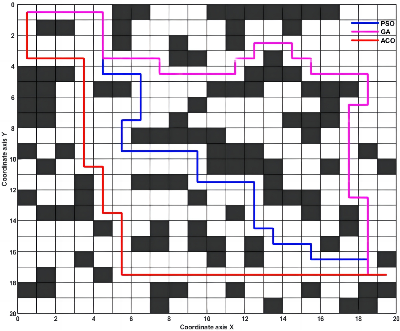
The path planning results based on PSO, GA and ACO after 50 iterations are shown in Figure 1. The path obtained by PSO occupies 38 grids and is turned 16 times. The path obtained by GA algorithm occupies 42 grids and is turned 18 times. The path obtained by ACO algorithm occupies 36 grids and is turned 7 times. The planning results show that ACO is better than PSO and GA under the same number of iterations, so it is more suitable for solving the path planning problem.
The selection operator in GA can ensure that all the selected individuals are excellent, but the mutation operator and crossover operators only introduce new individuals, and their operations cannot guarantee whether the new individuals are excellent. If the newly generated individuals are not sufficiently excellent, the introduction of new individuals will become an interference factor, which will slow down the search speed of GA. For PSO, the biggest problem in the application of graph theory path planning is that there is no unified prior knowledge of parameter setting (such as inertia weight, acceleration coefficient) and application background, resulting in unstable algorithm performance. ACO is also a type of feedback random search algorithm, but it relies on the pheromone (based on fitness function) left by ants for optimization. The initialization setting of the pheromone and the selection probability are closely related to the length of the path. This means that a shorter path attracts more ants. At the same time, the amount of residual pheromone is greater, which speeds up the optimization process. Therefore, ACO is chosen as the basic method to solve the problem of searching paths on graphs.
2.2 Dung Beetle Optimizer
Dung Beetle Optimizer (DBO) is a novel swarm intelligence algorithm that updates and optimizes the position of dung beetles by simulating four actions: ball rolling, breeding, foraging, and stealing.
(1) Ball-rolling dung beetle. When dung beetles move forward without obstacles, the position of dung beetles is updated as shown in Eq.(4). When dung beetles encounter obstacles, the tangential function is used to simulate the dancing behavior. The position updating formula is as follows Eq.(5).
where represents the position information of the dung beetle during the iteration. is a natural coefficient assigned to 1 or -1. is the random deflection coefficient of . is the random coefficient and is the position of the worst individual.
(2) Breeding. After the spawning area is determined based on Eq.(6), dung beetles will reproduce, and the position of the offspring dynamically changes, as shown in Eq.(7).
where represents the current local optimal position. , denotes the maximum number of iterations, is the current number of iterations, and represent the lower and upper bounds of the spawning area, and are two independent random vectors with a size of .
(3) The feeding area of dung beetles is determined based on Eq.(8). At this time, the position of dung beetles is updated as shown in Eq.(9).
where represents the global optimal position; is a D-dimensional random vector following a normal distribution; is the random vector within the range of .
(4) Stealing. The position of the thieving dung beetle is updated as follows:
where is a constant value. is a random vector subject to normal distribution with the size of .
3. Methodology
3.1 The framework of the two-layer path planning
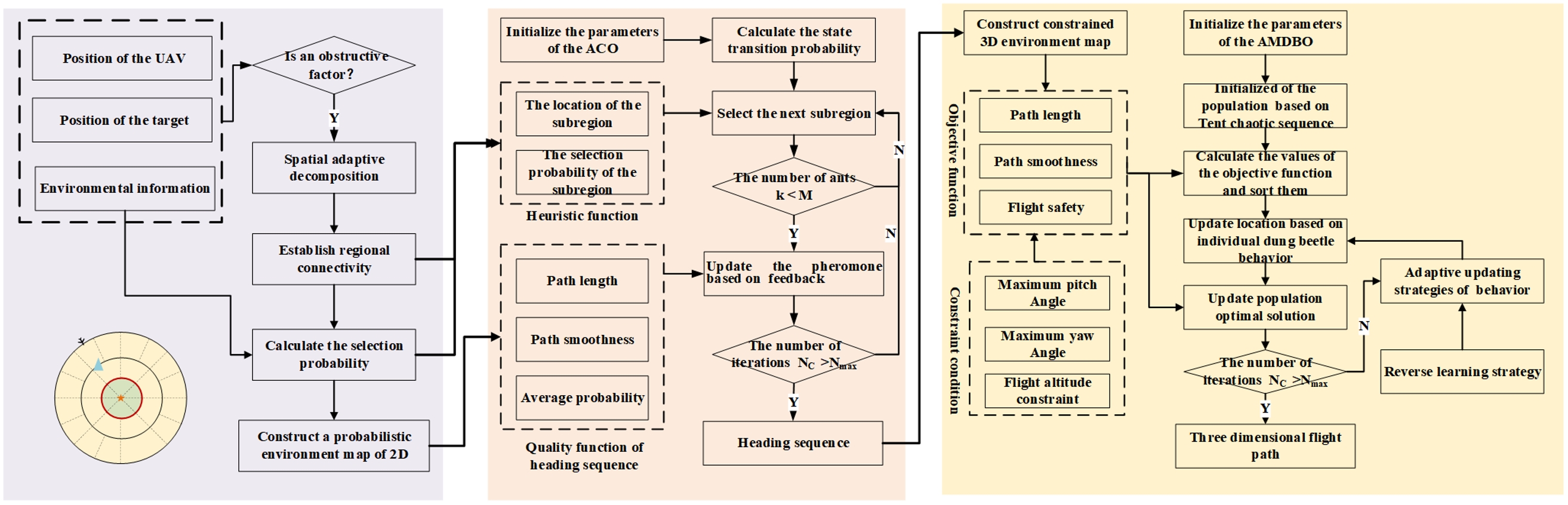
Facing the large airspace and complex interaction of environmental factors, planning a path directly from the overall three-dimensional environmental information poses challenges such as low efficiency and poor quality. The flowchart of the proposed two-layer trajectory planning is shown in Figure 2. The basic idea is to analyze the influence of multiple environmental factors on the heading within the airspace, and then construct an adaptive two-dimensional selection probability map through information fusion, and then propose an improved ant colony algorithm to carry out the first layer of coarse-grained heading sequence planning. This process aims to identify regions conducive to task execution. Subsequently, the spatial distribution of obstacles in the subregions is considered, and trajectory optimization is performed in the 3D space.
Heading planning and path planning are conducted within distinct layers of a unified framework, each with its specific focus. The heading planning phase prioritizes the assessment of the multi-dimensional environmental factors affecting the global path, thereby facilitating a coarse-grained heading planning approach. Conversely, path optimization aims to enhance the smoothness of the path while minimizing the path length, all while ensuring flight safety in accordance with heading space constraints and the maneuvering conditions applicable to unmanned aerial vehicles (UAVs). Path optimization is to improve path smoothness, flight safety and shorten path length with the maneuvering constraint conditions of UAV. However, they are closely related to each other. Trend planning provides a general framework and macroscopic direction guidance for path planning, while path planning is a fine design based on the existing heading to ensure that the UAV flight not only meets the predetermined macroscopic path, but also meets various constraints and performance requirements in the actual flight.
3.2 Construction of adaptive 2D probability map
3.2.1 Adaptive spatial decomposition strategy
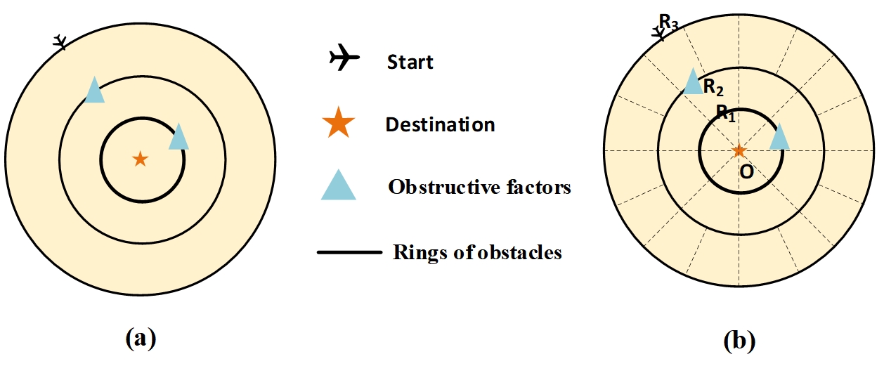
1) The coordinate system is built with the target as the center, and the distance between the initial position of the UAV and the target is the far boundary. Extraction of terrain, wind speed, and visibility within the airspace. Due to the wide range of airspace, an adaptive spatial distribution decomposition of airspace based on obstructive factors is proposed. Among them, the obstacle factor is the environmental factor that causes the UAV's flight direction to be impossible and the heading direction must be changed [28]. In this paper, elevation greater than 5200 m, visibility less than 0.8 km, and wind speed greater than 25 m/s, are considered as obstruction factors. As shown in Figure 3(a), there are two obstacle factors in the airspace, which is divided into three-ring layers.
2) To reduce the evaluation errors among sub-regions, each ring layer is divided into 32, 16, and 8 sub-regions from outer to inner layers. As illustrated in Figure 3(b), the first layer (o-R1) of the ring region is divided into eight sub-regions. The second layer of the ring region (R2-R1) is divided into 16 sub-regions. The third layer (R3-R2) is divided into 32 sub-regions.
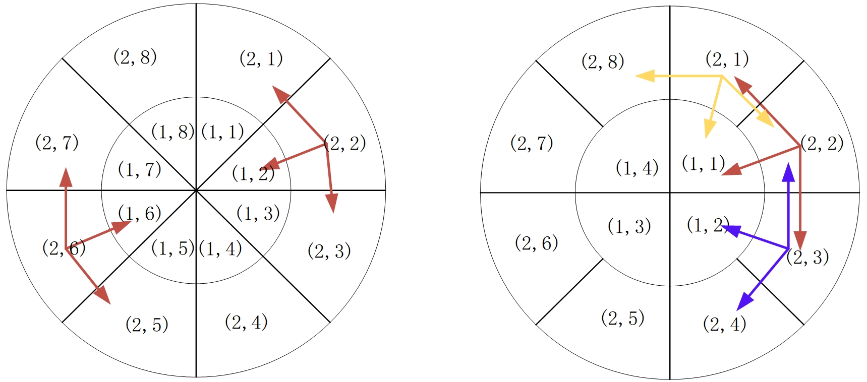
3) Connectivity of subregions. The represents the relative position between sub-regions, indicating that the current sub-region is located in the j-th discrete region of the i-th ring layer. There are only three choices from the current sub-region to the next sub-region. The connectivity of sub-regions is illustrated in Figure 4. If the numbers of sub-regions in two adjacent layers are the same, the next possible sub-regions are shown in Figure 4(a). If the numbers of sub-regions in two adjacent layers are different, the next sub-regions are demonstrated in Figure 4(b). Therefore, the mathematical description is shown in Eq.(11). There is no connectivity between the innermost sub-regions. The ring layers are unidirectionally connected, which can only be connected from the outer ring to the inner ring.
where are the total number of neutron regions in and layer respectively, , are -ary operation, is a ceiling operation.
3.2.2 Calculation of heading selection probability
During UAV flight operations, this study primarily considers the impacts of elevation, visibility, and wind speed on reconnaissance mission performance. Through information fusion, we subsequently evaluate the flight selection probability within each sub-region.
(1) Most UAVs adopt low-altitude penetration tactics, so the terrain elevation has a decisive effect on the heading. The lower the ground elevation, the stronger the shielding ability, and the greater the selection possibility .
(2) When the visibility is below 1.22 km, the clarity of vision is poor, which seriously threatens the flight safety of the UAV, and its flight direction selection is limited. When the visibility is between 1.22 km and 6 km, it significantly affects the clarity of vision and the degree of radar attenuation. When the visibility exceeds 6 km, the possibility of choosing the direction is higher.
(3) With the increase in wind speed, the control performance and maneuvering stability of the UAV deteriorate. Therefore, when selecting the flight direction, it often avoids regions with high wind speeds. When the wind speed is less than 1.5 m/s, it does not affect the UAV's flight, and the selection possibility is high. Wind speed starts to impact operational performance in the range of 1.5 m/s to 20 m/s, and the selection possibility decreases as wind speed increases. When the wind speed exceeds 30 m/s, it becomes unsafe to fly, and the selection possibility is low.
Combined with the grading standards of terrain and meteorology, this paper makes a fuzzy representation of environmental factors, as shown in Table 1.
|
0.8 | 0.6 | 0.4 | 0.2 | ||
|---|---|---|---|---|---|---|
| Altitude(m) | 600 | 600-2700 | 2700-4800 | 4800 | ||
| Visibility(Km) | 6 | 2.5-6 | 1.5-2.5 | 1.5 | ||
| wind speed(m/s) | 1.5 | 1.5-10 | 10-20 | 20 |
Then the calculation formula based on multi-source information fusion of the heading selection probability is shown in Eq.(12), where , represent the barrier area and total area of the subregion respectively.
3.3 Heading sequence planning based on IACO
The specific steps for searching the heading sequences in airspace based on the IACO are as follows:
(1) Initial ant colony parameters: colony number , maximum number of iterations , pheromone concentration factor , heuristic function factor , pheromone volatilization coefficient .
(2) Set the initial pheromone concentration to be uniform within each subregion and place all ants at the initial position of the drone as a starting point.
(3) According to the information in the 2D probability map, the transfer probability of ant from subregion to subregion is calculated, as shown in Eq(3).
(4) After all ants complete traversal of all feasible heading sequences, the pheromone on each subregion needs to be updated, as shown by the Eqs.(17-19). If ant does not pass the subregion sequence ,, the value is 0.
(5) If the current number of iterations reaches the upper limit, the search terminates. If it has not reached the limit, it proceeds to step (2) to continue iterating.
3.3.1 Heading planning objective function
The course of UAV is described by selecting the sub-region sequence set, .
The quality of feasible solution is evaluated from sequence length, possibility, and tortuosity. The length of the sequence is not only limited by the flight range of UAV, but also affects the flight time; a shorter sequence length results in a shorter flight time, which is crucial for completing the flight task efficiently. A higher mean probability of the sequence reduces the risk to the UAV. The sequence's tortuosity should be as smooth as possible due to flight maneuverability constraints. We propose that the direction sequence quality be evaluated according to Eq.(13).
where , , represent the length ratio, mean probability, tortuosity of sequence respectively. The calculation formulas are as shown in (14). And , , are the corresponding weights.
where represents total length of sequence sets, is the straight-line distance from the flight start point to the end point, . represents total probability of sequence sets, is the number of sub-regions in the course sequence set. is a constant, representing the maximum allowable direction tortuosity of UAV.
3.3.2 IACO
When the flight environment is complex, ACO is challenged due to the large search space when selecting the next region, leading to extended processing time and subpar real-time performance. To address this issue, an improved ant colony algorithm (IACO) is proposed.
(1) The new heuristic function is critical in inspiring ants to select nodes, directly affecting the solution quality. This new heuristic information considers the heading selection possibility of sub-regions and the distance between the sub-region and the flight destination. This allows for selecting sub-regions beneficial to the flight task, layer by layer.
where is the selection possibility of sub-region , and is the distance between the center of the sub-region and the flight end point, , , and are weights of two heuristic factors, and . The calculation of is shown in (16).
When the flight start point and end point are known, is a constant, and represents the distance between selected sub-region and flight end point. According to Eq.(16), the closer the last selected sub-region is to the flight endpoint, the greater the probability of selecting the sub-region, which reduces the search range and improves convergence speed.
(2) To solve the problem that the global pheromone update rule based on positive feedback cannot guide ants to search for the optimal solution in time, a new pheromone update strategy based on positive and negative feedback is constructed.
1) For ants searching for feasible solutions from the start to the end, the pheromones are updated based on positive feedback, as shown in Eqs. (17) and (18).
where is the quality evaluation value of the optimal sequence of current iteration. Compared with the traditional ACO, the search scope of ants in IACO is more concentrated in the neighborhood of the optimal heading sequence to achieve global optimization.
2) For ants that do not find a feasible solution, pheromone concentrations in corresponding subregions are updated based on negative feedback, as shown in Eq (19) .
where represents the distance between the last selected sub-region traversed by the deadlock ant and the flight end point. The attenuation of pheromone concentration is related to , which can not only avoid local optimization, but also avoid blind updating of global pheromone.
3.4 Path planning of 3D based on AMDBO
3.4.1 Objective function of 3D path planning
(1) The objective function of 3D path planning is similar to that of heading planning, as both have specific requirements for path length and smoothness. The difference lies in the calculation method. Moreover, flight path planning also takes into account the safety of UAVs.
where, , , are the three cost functions, , , are the corresponding weight coefficients, , are the scaling factors. The smaller the value of the objective function, the better the quality of the path.
1) Path length
where represents the number of track points, and represents the position of track point .
2) Path smoothness The 3D path design must meet its maximum climb angle and climb rate limits to ensure the curvature of the path and avoid sharp changes in direction and height fluctuations. represents the vector between two track points. Eqs.(22) and (23) respectively represent the yaw angle and the pitch angle . The cost function of path smoothness can be defined as Eq.(24).
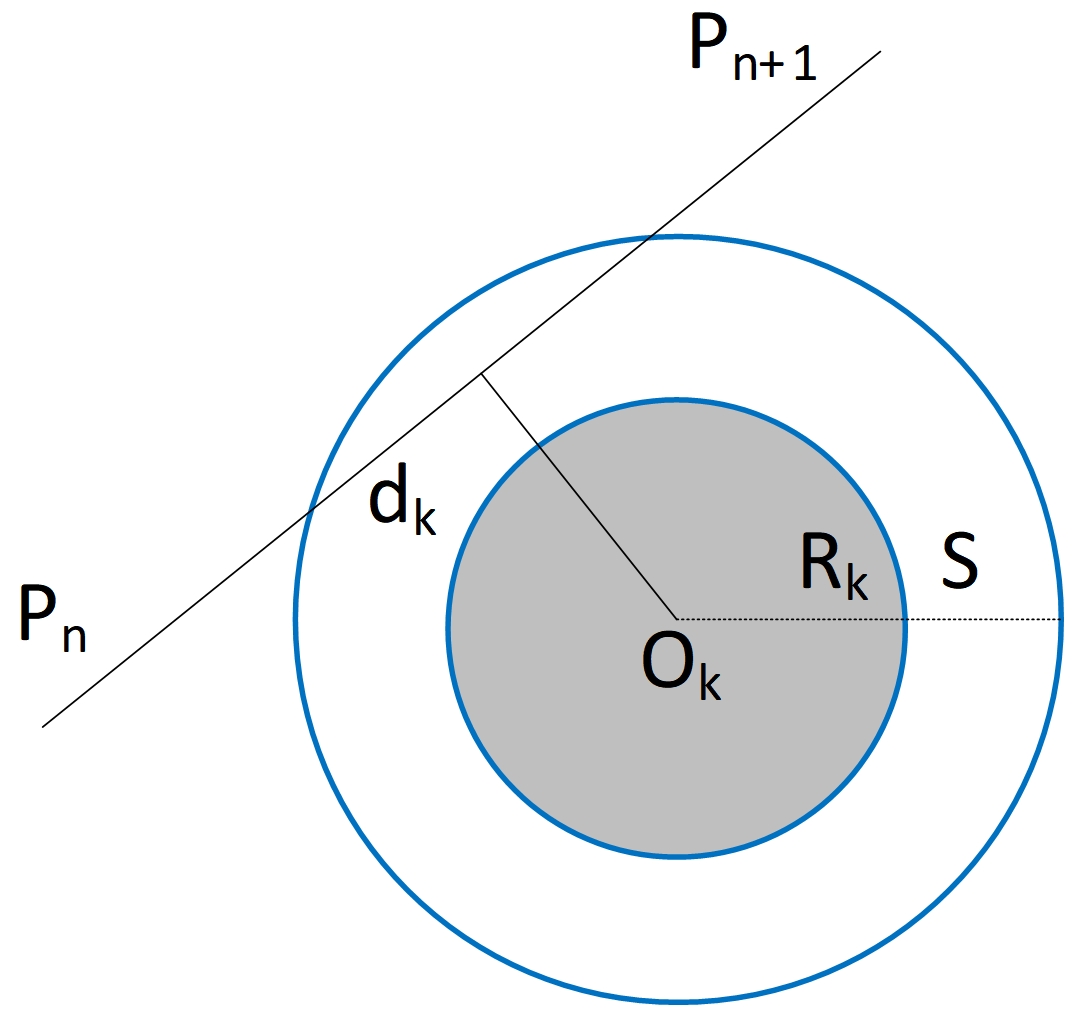
3) Path safety In order to ensure the safe flight of UAVs, a safety-oriented mechanism must be incorporated into the path planning process. As shown in Figure 5, there is an obstacle K in the airspace, whose central coordinate is and radius is . The vertical distance between the flight node of the UAV and the obstacle should be greater than the safety distance threshold m.
(2) constraint condition In order to achieve the feasibility of 3D path planning, constraints such as the flight performance of UAV must be considered, and the objective function exceeding the constraints should be punished with a penalty coefficient .
1) Maximum pitch angle. The pitch angle represents the angle of rotation around the X-axis. Constraining the angle change in the vertical direction when the UAV moves between adjacent nodes is crucial to prevent potential damage or crashes.
2) Maximum yaw angle. The yaw angle of the UAV involves its lateral rotation around the vertical axis (y-axis). The change in yaw angle must be strictly controlled to ensure that it stays within a safe range and prevents flight instability.
3) Flight altitude constraints. In order to ensure safe flight, the UAV should have a certain safe distance from the ground.
3.4.2 AMDBO
(1)Initialization strategy based on Tent Chaos When dealing with complex optimization problems, the original DBO randomly generates a population for initialization. However, this approach may lead to low population diversity, uneven population distribution, and rapid convergence to local optimal solutions. Tent Chaotic mapping offers better uniformity and correlation. Therefore, we utilize it as a new initialization method to enhance the population diversity of DBO. The formula is presented in Eq.(29).
(2)Reverse learning strategy
Since the global search ability of reproduction and stealing behavior decreases with the increase of iterations, a random reverse learning strategy is introduced to enhance the global search ability of these two behaviors.
where, is the reverse solution, and are D-dimensional vectors representing the lower and upper bounds of each dimension, and is the D-dimensional random vector of , is the current feasible solution.
(3) Adaptive population variation strategies In the original DBO, the ratio of the four behaviors in the population is not specified, and each individual can only perform one behavior. This limitation may lead to an inadequate search in the solution space or slow convergence. To address this issue, this paper proposes an adaptive behavior variation strategy.
1) Behavior variation strategy is based on the number of iterations. In this paper, the iteration number is used to simulate time, and the behavior variation of dung beetles is carried out every M iterations. This process changes the current behavior into the following behavior, allowing each dung beetle to perform four action behaviors. This approach maximizes the advantages of different behaviors and enhances the optimization ability.
2) Behavior variation strategy based on population similarity. Cosine similarity is introduced to measure population similarity, as shown in Eq.(31).
When the value is less than or greater than 0.5, individuals engaging in reproduction and foraging behaviors will transition into rolling ball behaviors. This transformation enhances the algorithm's global search capability, promoting species diversity. After finding the new best individual or reaching the iteration threshold of the variant individual, the variant individual will return to the original behavior and continue searching.
4. Experiments and analysis
In this section, we evaluate the performance of the proposed method. The structure of this section is as follows: we verify the effectiveness of the IACO in Section 4.1, discuss the optimization ability of AMDBO in Section 4.2, and analyze a two-layer path planning model in a simulated situational environment in Section 4.3.
4.1 Effectiveness analysis of IACO
4.1.1 Parameter setting
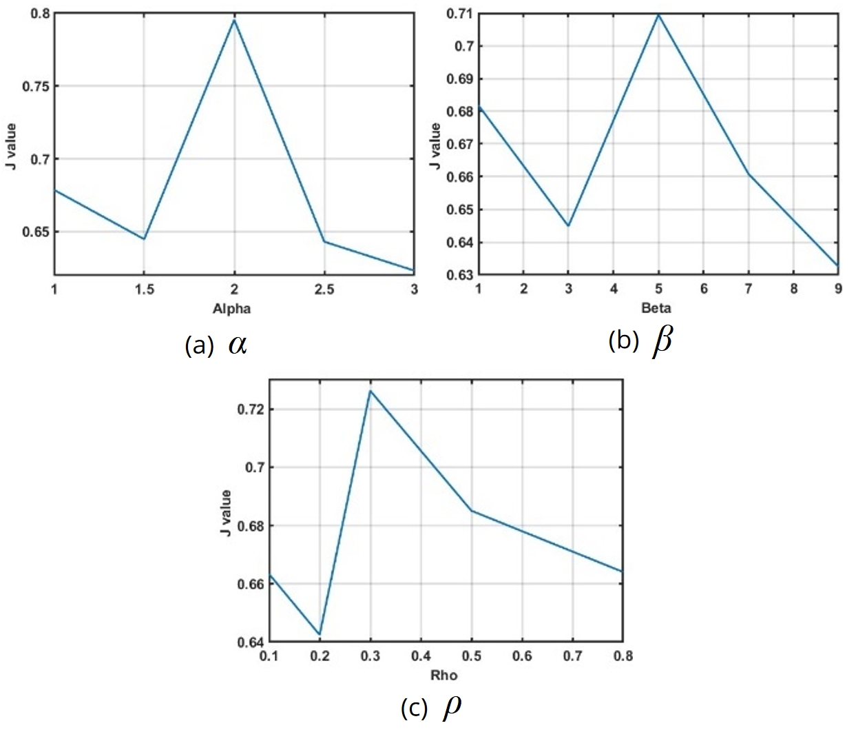
The setting of hyperparameters significantly impacts on the performance of evolutionary algorithms. Since there are no theoretical methods to determine the best parameter combination, hyperparameters must be fine-tuned and optimized through experiments to ensure the algorithm can find high-quality solutions efficiently [19]. In the ACO, pheromone and heuristic information play crucial roles in ant selection. Therefore, we focus on three key parameters: pheromone important parameter , heuristic factor important parameter , pheromone evaporation coefficient . The other initial parameters are: the total number of ants is 50, the maximum number of iterations is set to 100, and pheromone increase intensity coefficient .
This paper analyzes the influence of different values of , , and on the convergence results. Set a set of default values: , , . When analyzing the values of multiple parameters using the control variable method, one parameter's value is changed at a time while keeping the other parameters at their default values. To enhance the algorithm's robustness, the selected parameter combinations from each group are simulated in 20 random two-dimensional probability maps, and the average convergence values are compared and analyzed. The experimental results are shown in Figure 6.
It can be seen from the results in Figure 5 that when , , , the average convergence value reaches the maximum value, and the influence of on the average convergence result fluctuates the most. Therefore, the combination of , , is adopted in the subsequent experiments in this paper.
4.1.2 Contrastive analysis
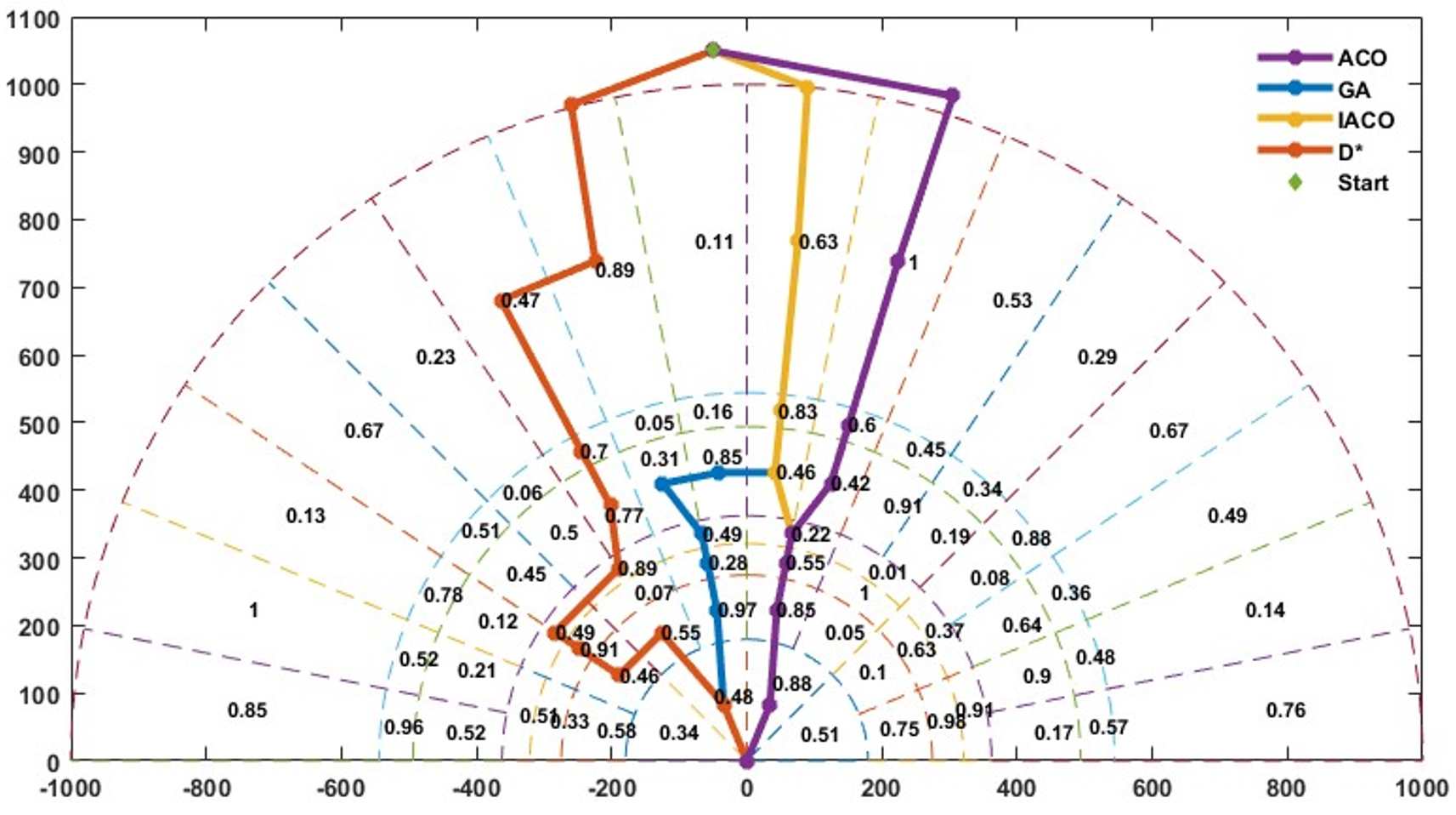
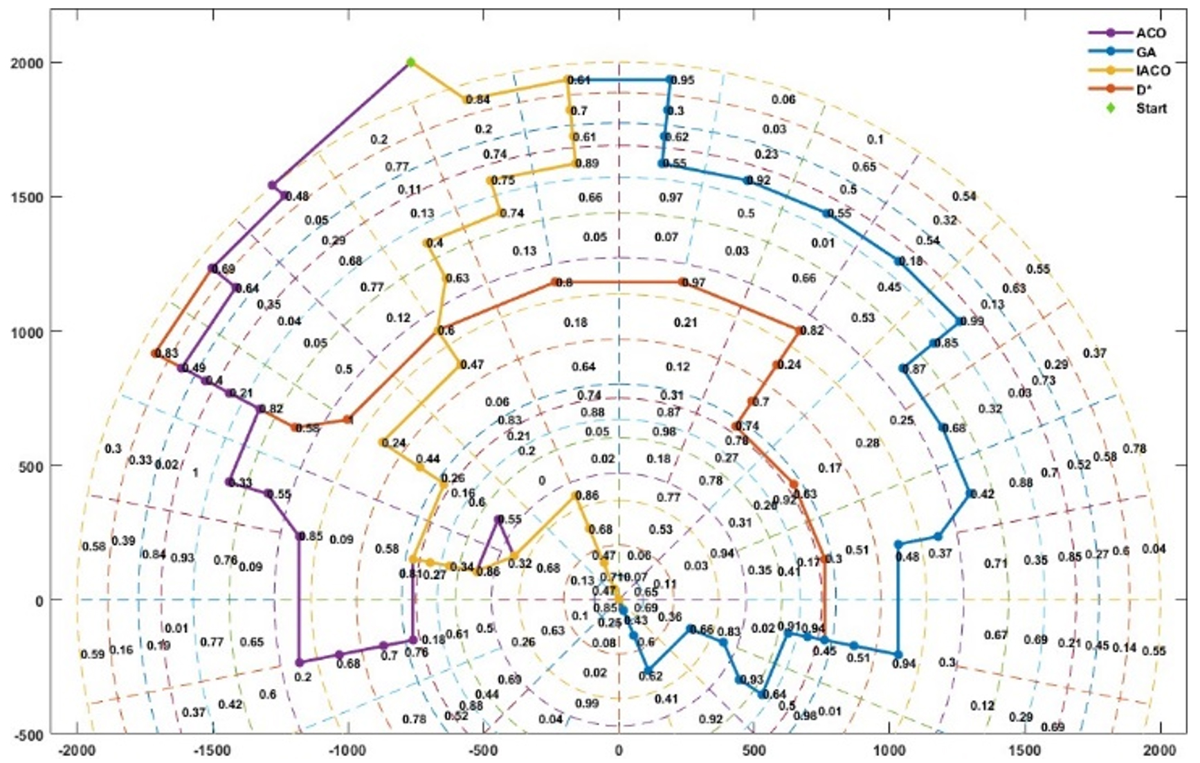
In order to further verify the effectiveness of heading planning based on IACO, the heading sequence is planned in the same 2D probability map (M1 and M2) based on D*, ACO, and GA. Figure 6 and Figure 7 display the planning results in M1 and M2, respectively.
In Figure 7, the heading sequence sets of ACO and IACO exhibit high similarity. The results of D* and the other three methods show the most significant difference. In Figure 8, the difference between the heading sequence sets of different methods is more significant than in M1, with the overall distribution ranging from 0° to 180° and 180° to 360°. The similarity between ACO and IACO is higher in the 8 ring layers near the target. The heading sequences obtained by GA and D* also align consistently within the 8 ring layers.
| Methods | ACO | GA | IACO | D* | |
|---|---|---|---|---|---|
| M1 | HL | 1402 | 1329 | 1161 | 1615 |
| HT | 0.375 | 0.592 | 0.322 | 0.977 | |
| HP | 0.614 | 0.625 | 0.614 | 0.568 | |
| M2 | HL | 5108 | 5717 | 4298 | 6787 |
| HT | 1.008 | 1.283 | 0.842 | 1.255 | |
| HP | 0.417 | 0.458 | 0.411 | 0.458 | |
| Function | Dimensionality | Search space | Theoretical value |
|---|---|---|---|
| 30 | [-100, 100] | 0 | |
| 30 | [-30, 30] | 0 | |
| 30 | [-500, 500] | -12569.5 | |
| 30 | [-600, 600] | 0 | |
| 2 | [-65.536, 65.536] | 1 | |
| 2 | [-5, 5] | 1.0316285 |
In this paper, the quality of the heading sequence is evaluated based on the length (HL), tortuous degree (HT), and selection possibility (HP/) of the heading sequence. The evaluation results of the heading sequence in Figure 7 and Figure 8 are presented in Table 2. It can be seen that the heading quality obtained by the four different algorithms in M2 is lower than that obtained in M1. The sequence length and sequence tortuous degree based on D* are the maximum values in the two maps, and the choice possibilities in the set of sub-regions vary widely. This result indicates that the heading sequence based on D* is trapped in a local optimum. IACO achieves the shortest length, the smallest tortuous degree, the largest average choice possibility in the two probability maps, and the highest comprehensive quality.
| F | Performance index | DBO | SSA | IGWO | AMDBO |
| AVE | 1.59E-109 | 1.63E-57 | 3.27E-29 | 3.67E-149 | |
| BEST | 7.35E-159 | 1.25E-146 | 1.68E-35 | 3.82E-196 | |
| STD | 7.68E-124 | 7.48E-63 | 9.34E-27 | 3.18E-147 | |
| AVE | 1.30E-03 | 1.42E-03 | 1.17E-03 | 7.48E-04 | |
| BEST | 4.05E-05 | 4.29E-04 | 1.68E-03 | 9.61E-05 | |
| STD | 1.10E-03 | 2.16E-03 | 1.84E-03 | 5.25E-04 | |
| AVE | -9.19E+03 | -8.57E+03 | -7.38E+03 | -1.17E+04 | |
| BEST | -1.23E+04 | -9.64E+03 | -1.07E+04 | -1.26E+04 | |
| STD | 1.95E+03 | 5.21E+02 | 1.62E+03 | 9.93E+02 | |
| AVE | 1.15E-13 | 0.00E+00 | 3.87E-03 | 0.00E+00 | |
| BEST | 0.00E+00 | 0.00E+00 | 0.00E+00 | 0.00E+00 | |
| STD | 6.27E-13 | 0.00E+00 | 6.41E-03 | 0.00E+00 | |
| AVE | 1.30E+00 | 5.03E+00 | 9.98E-01 | 1.16E+00 | |
| BEST | 9.98E-01 | 9.98E-01 | 9.98E-01 | 9.98E-01 | |
| STD | 6.97E-01 | 5.17E+00 | 1.80E-16 | 4.58E-01 | |
| AVE | -1.03E+00 | -1.03E+00 | -1.03E+00 | -1.03E+00 | |
| BEST | -1.03E+00 | -1.03E+00 | -1.03E+00 | -1.03E+00 | |
| STD | 4.85E-16 | 5.46E-16 | 8.14E-16 | 3.92E-16 |
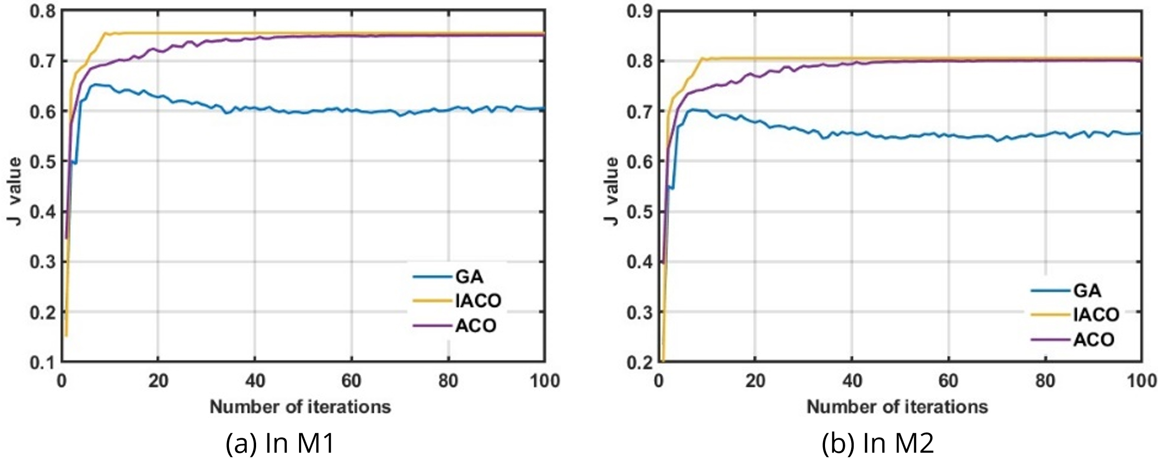
In addition, the convergence of GA, ACO, and IACO in the two maps is compared, as shown in Figure 9. The convergence quality and convergence speed based on the three algorithms in M2 are not as good as in M1. The convergence rate of GA is slow, and the convergence value of GA in M2 remains stable at a low level, indicating that GA also gets trapped in local optima. The main reason is that the mutation and crossover operators in GA cannot guarantee the quality of new individuals, thereby slowing down the optimization process. In comparison, ACO and IACO exhibit faster convergence speeds and higher quality. This result shows that ACO and IACO are more suitable for solving graph search problems.
| F | Performance index | DBO1 | DBO2 | DBO3 | AMDBO |
|---|---|---|---|---|---|
| AVE | 0.001158 | 0.000597 | 0.000885 | 0.001214 | |
| BEST | 0.000125 | 8.40E-05 | 5.26E-05 | 0.000194 | |
| STD | 0.001005 | 0.000548 | 0.000647 | 0.000936 | |
| AVE | 0.000784 | 0.000837 | 0.000553 | 0.000921 | |
| BEST | 0.000307 | 0.000307 | 0.000307 | 0.000307 | |
| STD | 0.000412 | 0.00039 | 0.000354 | 0.000498 | |
| AVE | -1.03163 | -1.03163 | -1.03163 | -1.03163 | |
| BEST | -1.03163 | -1.03163 | -1.03163 | -1.03163 | |
| STD | 6.45E-16 | 1.10E-15 | 5.61E-16 | 5.98E-16 |
The convergence performance based on IACO in the two maps is the best, converging to 0.815 and 0.755 in the 8th and 11th iterations, respectively. The results show that the heading planning based on the IACO can provide reliable decision support for the subsequent 3D path planning.
4.2 Effectiveness analysis of AMDBO
4.2.1 Test analysis based on benchmark functions
Compared with heading prediction in a 2D map, the algorithm's global search capability and search efficiency are more critical for the precise planning of a 3D path. DBO, Improved Grey Wolf Optimizer (IGWO), and Sparrow Search Algorithm (SSA) are comparisons to verify the optimization performance of AMDBO. Six functions with different optimal characteristics are compared, and their specific details are presented in Table 3. F1 and F2 are single-peak reference functions that are used to evaluate the algorithm's single-objective solving capability. F3-F4 represent multi-modal reference functions, while F5-F6 are mixed reference functions that assess the algorithm's ability to escape local optima.
(1) Performance analysis In order to enhance the reliability of the experimental results, this paper adopts a consistent experimental setting by fixing the population size of each algorithm at 30 and the number of iterations at 500. Thirty independent experiments are performed on each function to obtain the target solution under each run. The average value (AVE), best value (BEST), and standard deviation (STD) are then calculated. These values serve as indicators to evaluate the reliability and stability of the optimization algorithm. Table 4 displays the test results of the four optimization algorithms on the six test functions.
The AVE, BEST, and STD in F1 based on AMDBO are superior to the other three algorithms. When compared with the test results of F2, it is evident that the BEST of AMDBO is 57.76% lower than that of DBO, but the AVE and STD of AMDBO are 73.80% and 109.52% higher than those of DBO, respectively. Regarding the overall performance of the two single-peak functions, the overall performance of AMDBO is better than that of other three algorithms. The STD of AMDBO is slightly lower than that of SSA on F4. However, the AVE and the BEST of AMDBO are the highest, and the accuracy is greater than that of DBO and IGWO in F3 and F4. In F5 and F6, the best values of the four algorithms can achieve the theoretical optimal solution. Although the AVE and STD of AMDBO are slightly lower than IGWO on F5, they are superior to SSA and DBO. Additionally, the STD of AMDBO in F6 outperforms the other three algorithms.
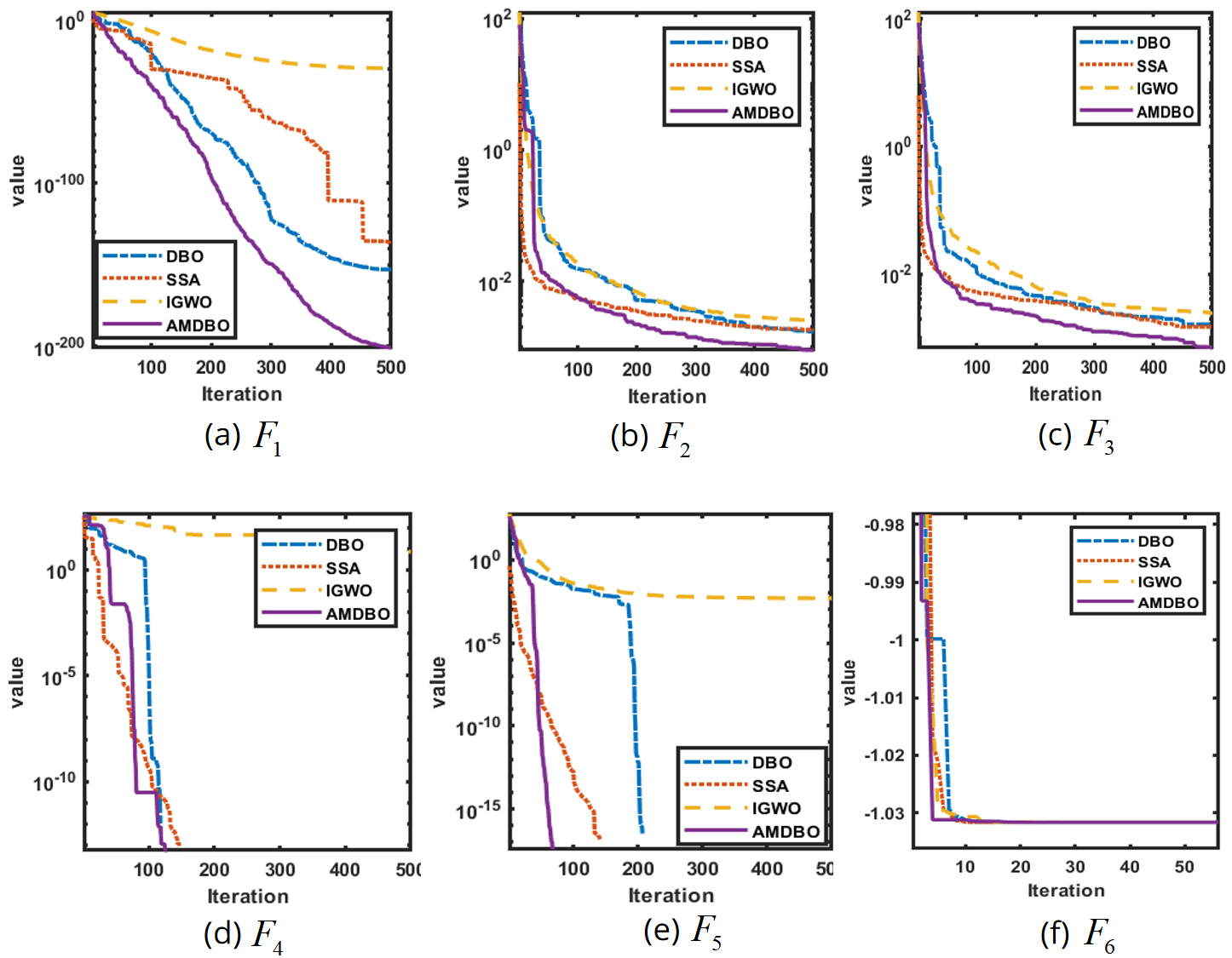
Figure 10 illustrates the average convergence curves of 4 algorithms in 30 independent tests across 6 test functions. It can be seen that AMDBO achieves a higher objective function value within the same number of iterations during single-objective optimization. It exhibits the fastest optimization speed and the highest convergence accuracy. AMDBO can swiftly escape local optimal solutions in multi-objective optimization, leading to faster convergence with fewer iterations.
To sum up, the AVE and BEST tested by AMDBO on the test functions are mostly better than the other three algorithms. With the same number of iterations, the optimization accuracy of AMDBO is higher. Most test results of the DBO algorithm are better or even superior to the SSA and IGWO, but worse than AMDBO.
4.2.2 Ablation Study
AMDBO introduces three improvement strategies to enhance the DBO algorithm. By implementing these strategies, three different algorithms derive through individual enhancements to DBO. The algorithms are as follows: 1) DBO1, which incorporates the Tent Chaos Initialization strategy. 2) DBO2, which integrates the reverse learning strategy of breeding and stealing. 3) DBO3, which includes the adaptive mutation strategy. These four algorithms are evaluated on test functions , and the AVE, BEST and STD of each algorithm are calculated after 30 independent runs. The experimental results are presented in Table 5.
In summary, the average optimization accuracy of a single improved strategy is higher than that of DBO. However, its variance is worse than that of DBO in test functions, indicating that the stability of a single improved strategy is insufficient. Compared with DBO, the performance indicators of AMDBO are improved, indicating that the comprehensive improvement of the three strategies is effective.
4.3 Effectiveness analysis of path planning model
4.3.1 Simulation scene test
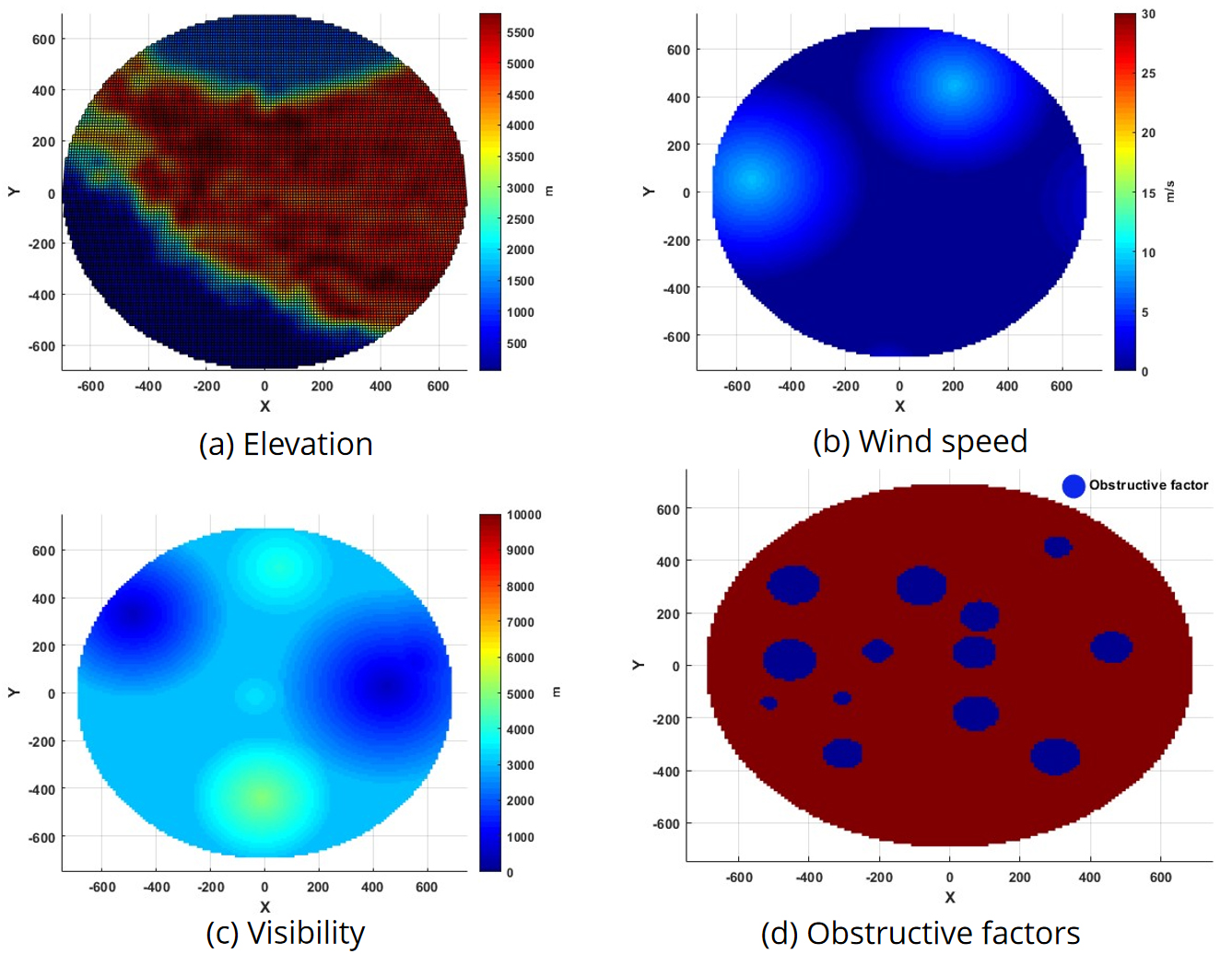
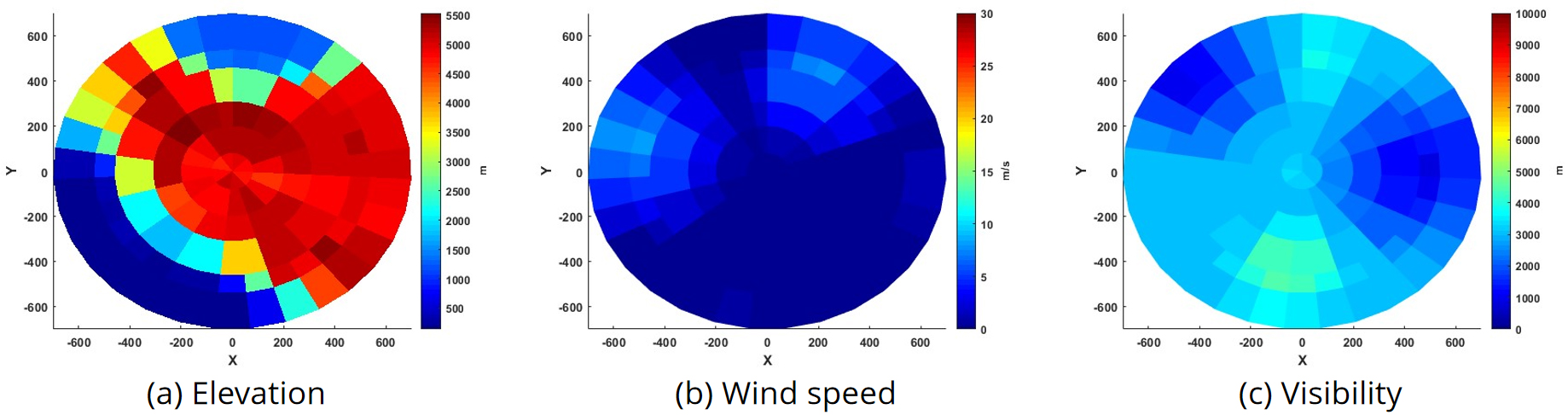
Taking the endpoint as the center of the circle and the distance between the starting point (-674,156) and the endpoint as the radius, the environmental information such as elevation, visibility, wind speed, and obstruction factors in this vast airspace is simulated, as shown in Figure 11. Then, the UAV trajectory is planned based on the fused multi-source environmental information.
According to the spatial distribution of obstacle factors in Figure 11(d), the airspace is adaptively decomposed into 80 km, 200 km, 310 km, 460 km, 540 km, and 700 km. The environmental situation information in each sub-area is shown in Figure 12. Comparing it with the actual scene grid information in Figure 11(a-c), it can be observed that the decomposition method accurately reflects the changing trend of environmental information while reducing the number of subregions. The results indicate that the adaptive spatial decomposition method effectively addresses the issue of sparse environmental information.
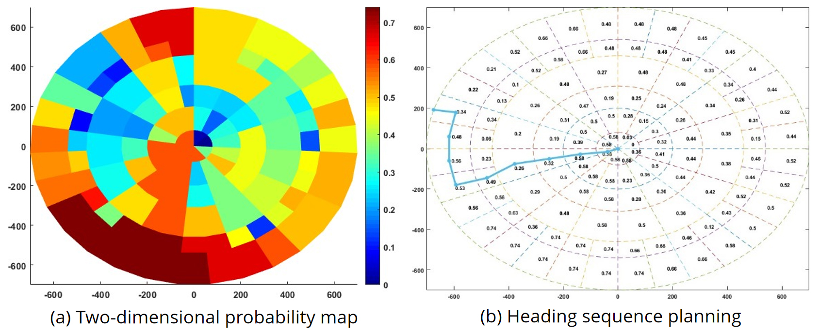
Based on Eq.(12), the 2D probability map is constructed, as shown in Figure 13(a). The IACO is used to search the heading sequence, and the result is shown in Figure 13(b). The flight direction gradually changed from 292.5° to 225°-270°. The average choice possibility of the route is 0.46, and the minimum value is 0.32, indicating that flight safety is relatively reliable. The tortuous degree of the heading sequence is 0.52, and the length is 1075.1 km, which is relatively smooth and short.
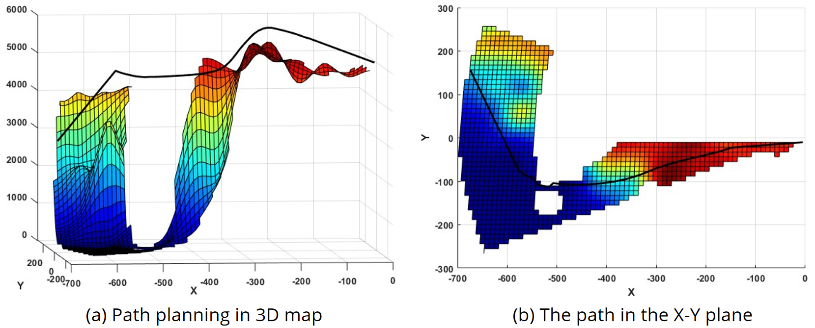
The AMBDO is used to plan a 3D path in regions where the heading sequence is located. The results are shown in Figure 14. The length of the 3D path is 4536 km, the average height is 4674 m, and the average tortuosity is 7.9. The 3D path is relatively smooth, and obstructions can be avoided.
4.3.2 Contrastive analysis
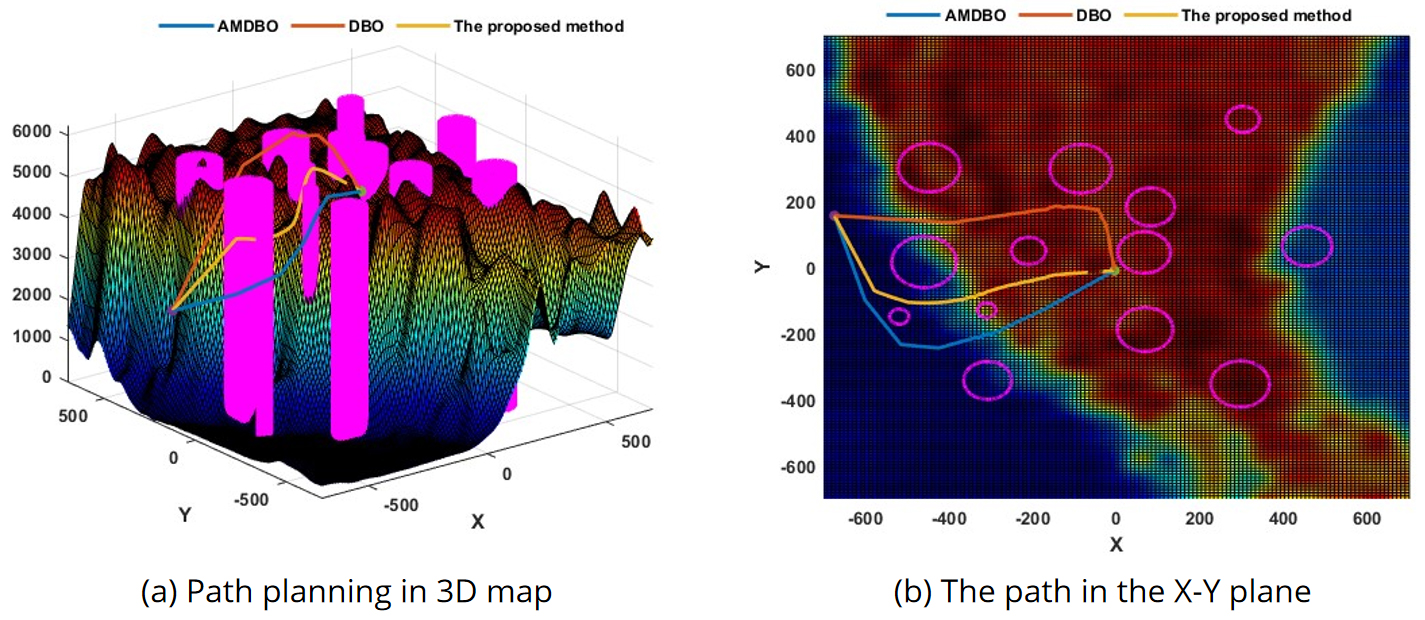
In order to verify the advantages of the two-layer path planning model proposed in this paper, the AMDBO is used to plan the path directly in 3D space. The planning results are shown in Figure 15. It is evident from Figure 13 that feasible paths are successfully planned using the three methods. The paths generated by DBO are distributed in regions with elevated terrain. To ensure a safe distance from the ground, the resulting paths are at a higher altitude and exhibit a greater tortuous degree. The other two methods exhibit a similar path trajectory, opting to first navigate towards lower-lying areas.
In this paper, path quality is evaluated based on path length (L), average flight height (H), tortuosity (T), and minimum distance from obstacles (Df). The evaluation results for the three methods are presented in Table 6. The path generated by DBO is shorter than that of AMDBO, but it exhibits high tortuosity. The path produced by AMDBO has a lower average height, enhancing its ability for concealed flight, but it has a longer path length. The proposed method demonstrates the shortest path length and tortuosity, with a flight altitude comparable to other methods, resulting in the highest overall quality.
| Indicators | AMDBO | DBO | Proposed method |
|---|---|---|---|
| L (km) | 4825 | 4536 | 3753 |
| H (m) | 4466 | 4843 | 4674 |
| T | 16 | 42.2 | 7.9 |
| Df (km) | 2.14 | 1.13 | 2.23 |
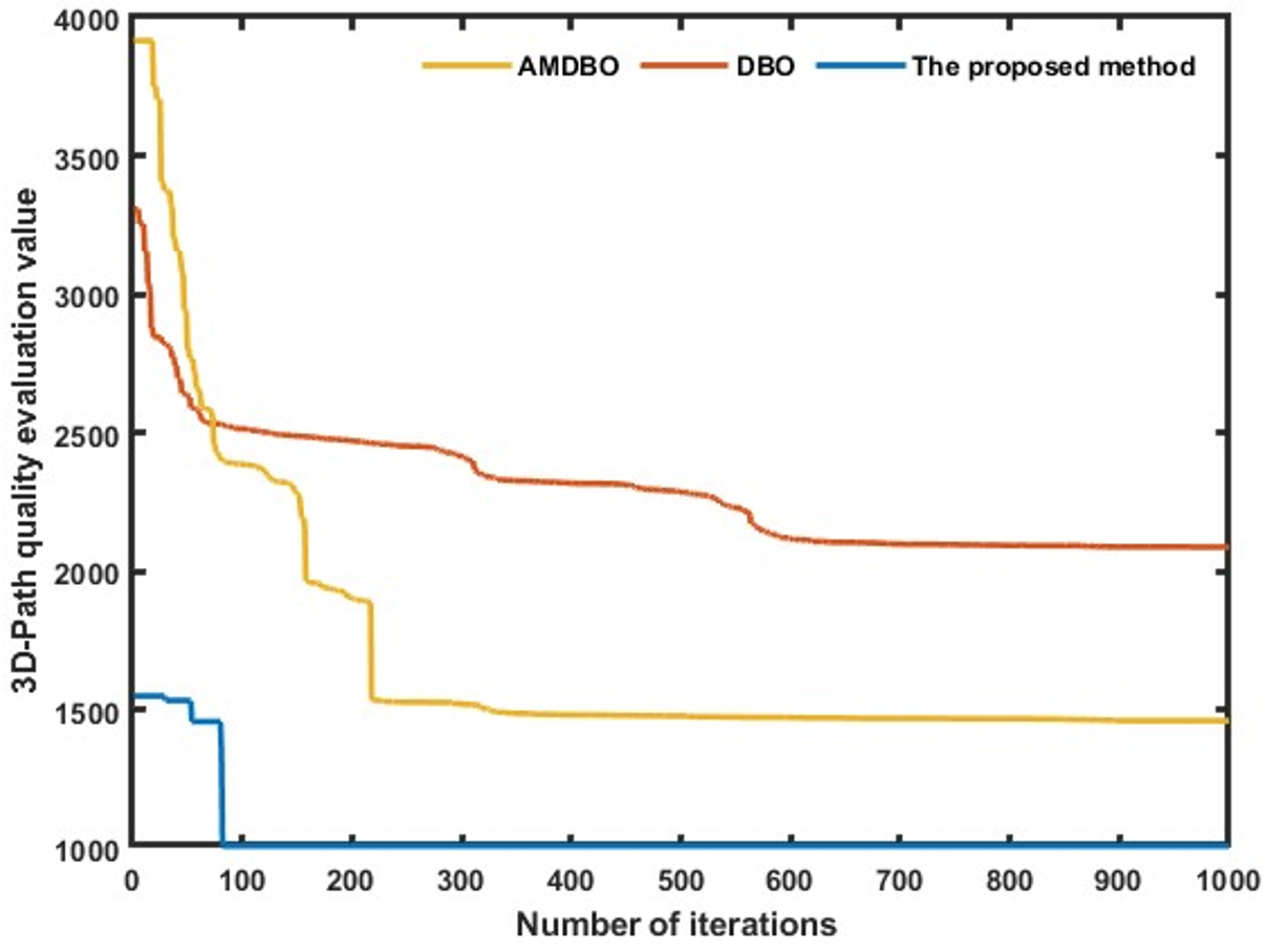
In addition, the convergence curves of the two models are compared, as shown in Figure 16. The DBO jumps out of the local solution twice and finally converges to 2091 in the 574th iteration. Although the objective function value of AMDBO is higher than that of DBO in the 1-73 iterations, its convergence rate is faster, and the convergence value is lower than that of DBO. The initial value of the proposed method is close to the convergence value of AMDBO and converges to 1007 at the 81st iteration. Compared with AMDBO and DBO, the convergence speed of the proposed method is increased by 75% and 85.89%, respectively, and the convergence values decreased by 31.87% and 52.05%, respectively.
Based on the above analysis, the two-layer path planning framework proposed in this paper can not only fully consider the impact of the environment on the UAV mission but also carry out fine path planning combined with the maneuvering performance of the UAV. Simultaneously, the environmental information of large airspace is analyzed layer by layer from fine-grained to coarse-grained to fine-grained. This effectively reduces the computational complexity and the execution efficiency of the optimization algorithm, thus improving the efficiency and quality of the flight path planning.
5. Conclusion
This paper establishes a dual-layer path planning model by integrating: (1) an adaptive 2D probability map based on information fusion, (2) an enhanced ant colony algorithm, and (3) an improved dung beetle optimizer. The proposed framework achieves phased trajectory planning for UAVs in large-scale airspace environments, followed by comprehensive effectiveness validation. The IACO demonstrates superior convergence quality and speed compared to ACO, GA, and D* in the 2D probability map for heading planning, facilitating reliable decision-making for subsequent 3D path planning. Compared with the optimization results of DBO, SSA, and IGWO in multi-type functions, the AMDBO proposed in this paper demonstrates strong global search ability and search efficiency. It provides theoretical support for the precise planning of 3D paths for UAVs in vast airspace. Comparing the planning results of AMDBO, DBO, the proposed method under the same simulation scenario, the proposed method shows a 75% and 85.89% increase in convergence speed and a 31.87% and 52.05% decrease in convergence values, respectively. These results indicate that the two-layer path planning model can effectively reduce computational complexity and optimize algorithm efficiency.
This paper focuses on studying the global path-planning method of UAVs based on macroscopic modal constraints. However, it faces challenges when it comes to environments with dense and highly dynamic obstacles. Future research will further study the online path planning for UAVs in such complex environments.
Data Availability Statement
Funding
Conflicts of Interest
Ethical Approval and Consent to Participate
References
- Sepulveda, E., & Smith, H. (2017). Technology challenges of stealth unmanned combat aerial vehicles. The Aeronautical Journal, 121(1243), 1261-1295.
- Qin, J., & Wu, X. (2016, October). Modeling and simulation on the earliest launch time of ship-to-air missile of warship formation in cooperative air-defense. In 2016 IEEE Advanced Information Management, Communicates, Electronic and Automation Control Conference (IMCEC) (pp. 375-379). IEEE.
- Gao, Y., Li, D. S., & Zhong, H. (2020). A novel target threat assessment method based on three-way decisions under intuitionistic fuzzy multi-attribute decision making environment. Engineering Applications of Artificial Intelligence, 87, 103276.
- Zhang, R., Chai, R., Chai, S., Xia, Y., & Tsourdos, A. (2023). Design and practical implementation of a high efficiency two-layer trajectory planning method for AGV. IEEE transactions on industrial electronics, 71(2), 1811-1822.
- Bashir, N., Boudjit, S., Dauphin, G., & Zeadally, S. (2023). An obstacle avoidance approach for UAV path planning. Simulation modelling practice and theory, 129, 102815.
- Ren, Z., Rathinam, S., Likhachev, M., & Choset, H. (2022). Multi-objective path-based D* lite. IEEE Robotics and Automation Letters, 7(2), 3318-3325.
- Chong, L., Jian, L., & XueQuan, L. (2020). Static rectangle expansion A* algorithm for pathfinding. IEEE Transactions on Games, 14(1), 23-35.
- Ali, H., Xiong, G., Haider, M. H., Tamir, T. S., Dong, X., & Shen, Z. (2023). Feature selection-based decision model for UAV path planning on rough terrains. Expert Systems with Applications, 232, 120713.
- Diao, Q., Zhang, J., Liu, M., & Yang, J. (2023). A Disaster Relief UAV Path Planning Based on APF-IRRT* Fusion Algorithm. Drones, 7(5), 323.
- Zhang, J., An, Y., Cao, J., Ouyang, S., & Wang, L. (2023). UAV trajectory planning for complex open storage environments based on an improved RRT algorithm. IEEE Access, 11, 23189-23204.
- Hao, G., Lv, Q., Huang, Z., Zhao, H., & Chen, W. (2023). Uav path planning based on improved artificial potential field method. Aerospace, 10(6), 562.
- Liu, J., Yan, Y., Yang, Y., & Li, J. (2024). An Improved Artificial Potential Field UAV Path Planning Algorithm Guided by RRT Under Environment-aware Modeling: Theory and Simulation. IEEE Access.
- Wu, J., Wang, H., Wang, Y., & Liu, Y. (2021). UAV reactive interfered fluid path planning. Acta Automatica Sinica, 47(1), 1-16.
- Yang, T., Yang, F., & Li, D. (2024). A New Autonomous Method of Drone Path Planning Based on Multiple Strategies for Avoiding Obstacles with High Speed and High Density. Drones, 8(5), 205.
- Dewangan, R. K., Shukla, A., & Godfrey, W. W. (2019). Three dimensional path planning using Grey wolf optimizer for UAVs. Applied Intelligence, 49, 2201-2217. https://link.springer.com/article/10.1007/s10489-018-1384-y
- Hu, K., & Mo, Y. (2024). A novel unmanned aerial vehicle path planning approach: sand cat optimization algorithm incorporating learned behaviour. Measurement Science and Technology, 35(4), 046203. https://iopscience.iop.org/article/10.1088/1361-6501/ad1977/meta
- Zheng, R. Z., Zhang, Y., & Yang, K. (2022). A transfer learning-based particle swarm optimization algorithm for travelling salesman problem. Journal of Computational Design and Engineering, 9(3), 933-948.
- Xue, J., & Shen, B. (2023). Dung beetle optimizer: A new meta-heuristic algorithm for global optimization. The Journal of Supercomputing, 79(7), 7305-7336. https://link.springer.com/article/10.1007/s11227-022-04959-6
- Miao, C., Chen, G., Yan, C., & Wu, Y. (2021). Path planning optimization of indoor mobile robot based on adaptive ant colony algorithm. Computers & Industrial Engineering, 156, 107230.
- Shen, Q., Zhang, D., Xie, M., & He, Q. (2023). Multi-strategy enhanced dung beetle optimizer and its application in three-dimensional UAV path planning. Symmetry, 15(7), 1432.
- Lyu, L., Jiang, H., & Yang, F. (2024). Improved Dung Beetle Optimizer Algorithm with Multi-Strategy for global optimization and UAV 3D path planning. IEEE Access.
- Jiachen, H., & Li-hui, F. (2024). Robot path planning based on improved dung beetle optimizer algorithm. Journal of the Brazilian Society of Mechanical Sciences and Engineering, 46(4), 235. https://link.springer.com/article/10.1007/s40430-024-04768-3
- Wai, R. J., & Prasetia, A. S. (2019). Adaptive neural network control and optimal path planning of UAV surveillance system with energy consumption prediction. IEEE Access, 7, 126137-126153.
- Liu, Y., Zheng, Z., Qin, F., Zhang, X., & Yao, H. (2022). A residual convolutional neural network based approach for real-time path planning. Knowledge-Based Systems, 242, 108400.
- Luo, X., Wang, Q., Gong, H., & Tang, C. (2024). UAV path planning based on the average TD3 algorithm with prioritized experience replay. IEEE Access.
- Zhou, C., Gu, S., Wen, Y., Du, Z., Xiao, C., Huang, L., & Zhu, M. (2020). The review unmanned surface vehicle path planning: Based on multi-modality constraint. Ocean Engineering, 200, 107043.
- Huang, Z. M., Chen, W. N., Li, Q., Luo, X. N., Yuan, H. Q., & Zhang, J. (2020). Ant colony evacuation planner: An ant colony system with incremental flow assignment for multipath crowd evacuation. IEEE Transactions on Cybernetics, 51(11), 5559-5572.
- Yang, T., Yang, F., & Li, D. (2022). An Air Target Course Prediction Method Based on Sub-Regions Divide and Conquer With Double Variable Weight. IEEE Access, 10, 117871-117885.
Cite This Article
Article Metrics
Citations:Article Access Statistics:
Publisher's Note
ICCK stays neutral with regard to jurisdictional claims in published maps and institutional affiliations.
Rights and Permissions

Copyright © 2024 by the Author(s). Published by Institute of Central Computation and Knowledge.
This article is an open access article distributed under the terms and conditions of the Creative Commons Attribution (CC BY) license.