Complex Evidence Theory for Multisource Data Fusion

Fuyuan Xiao; Junhao Wen; Witold Pedrycz; Masayoshi Aritsugi

doi:10.62762/CJIF.2024.999646

Abstract

Data fusion is a prevalent technique for assembling imperfect raw data coming from multiple sources to capture reliable and accurate information. Dempster–Shafer evidence theory is one of useful methodologies in the fusion of uncertain multisource information. The existing literature lacks a thorough and comprehensive review of the recent advances of Dempster– Shafer evidence theory for data fusion. Therefore, the state of the art has to be surveyed to gain insight into how Dempster–Shafer evidence theory is beneficial for data fusion and how it evolved over time. In this paper, we first provide a comprehensive review of data fusion methods based on Dempster–Shafer evidence theory and its extensions, collectively referred to as classical evidence theory, from three aspects of uncertainty modeling, fusion, and decision making. Next, we study and explore complex evidence theory for data fusion in both closed world and open world contexts that benefits from the frame of complex plane modelling. We then present classical and complex evidence theory framework-based multisource data fusion algorithms, which are applied to pattern classification to compare and demonstrate their applicabilities. The research results indicate that the complex evidence theory framework can enhance the capabilities of uncertainty modeling and reasoning by generating constructive interference through the fusion of appropriate complex basic belief assignment functions modeled by complex numbers. Through analysis and comparison, we finally propose several challenges and identify open future research directions in evidence theorybased data fusion.

Graphical Abstract

Complex Evidence Theory for Multisource Data Fusion

Click image to view fullscreen

Keywords

multisource data fusion Dempster-Shafer evidence theory complex evidence theory quantum evidence theory uncertainty modeling conflict management belief function decision making pattern classification

1. Introduction

With the development of the information age, large amounts of data are being generated, gathered and disposed. Interfering based on solely on single source is no longer sufficient. Data fusion, also known as multisource data fusion, is a necessary technique to assemble various kinds of data from multiple sources to capture reliable and accurate information [1, 2, 3, 4]. Nevertheless, uncertain, imprecise, imbalance, and incomplete or even false data are inevitable on account of the impacts of the environment and the complexity of the goals [5, 6, 7]. Such kinds of problems increase difficult to multisource data fusion. To improve the performance of the fusion system, various data fusion methods have been presented [8, 9], and applied in a wide variety of areas [10, 11, 12, 13, 14], including artificial intelligence, target tracking and recognition, smart engineering management, IoT systems, financial systems, medical diagnosis, and so on [15, 16, 17].

Existing works provide an overview of the effort related to data fusion from different perspectives. Some papers [18, 19] investigate data fusion in smart Internet of Things (IoT). Some papers [20] investigate multisensor data fusion techniques. A comprehensive survey on data fusion in remote sensing is presented in [21]. Some papers [22] investigate data fusion in machine learning. A survey in [23] presents mobile agent itinerary planning for information fusion in wireless sensor networks. A survey on information fusion for edge intelligence is presented in [24]. A recently published survey conducts a comprehensive statistical analysis of the current theoretical and application achievements of multisource information fusion [25]. Dempster–Shafer evidence theory (DSET) [26, 27] is one of useful methodologies in the fusion of uncertain multi-source information [28]. To the best of our knowledge, although researchers have conducted reviews and surveys of data fusion from different perspectives, no attempt has been made to provide a comprehensive overview on the DSET for data fusion by carefully analyzing the abovementioned data fusion literature.

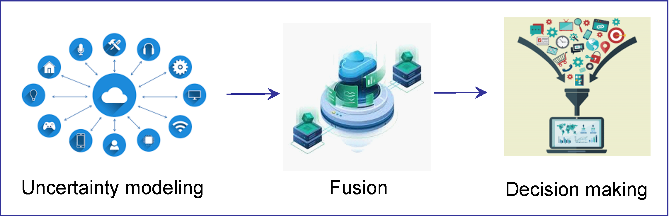
Therefore, in this paper, a comprehensive and systematic survey on data fusion in DSET is conducted. We first review the basic concepts and knowledge of classical DSET, then study the axioms of Dempster's rule of combination and the characteristics of DSET that are desirable for data fusion. Whereafter, we review classical DSET and its extensions, collectively referred to as classical evidence theory, for data fusion from three aspects of uncertainty modeling, fusion, and decision making. Next, we explore complex evidence theory for data fusion in both closed world and open world contexts that benefits from the frame of complex plane modelling. After that, we present classical and complex evidence theory framework-based multisource data fusion algorithms. These algorithms are applied to pattern classification to demonstrate their applicability through comparison with other related well-known methods. Finally, we discuss challenges and open directions for future research. The objectives of this work are to: 1) offer a general and synthetic review of classical and complex evidence theories; 2) provide a profound analysis and discussion of existing work in classical and complex evidence theory framework-based data fusion domains; and 3) identify remaining challenges and open directions for future research in this field.

The paper is organized as follows. Section 2 reviews classical DSET and its typical generalized theories. In Section 3, we analyze classical evidence theory for data fusion. In Section 4, we study and explore complex evidence theory for data fusion in both closed and open world contexts. In Section 5, classical and complex evidence theory framework-based multisource data fusion algorithms are presented. In Section 6, several challenges and open future research directions are discussed. Finally, Section 7 concludes this work.

2. Review of Classical DSET and Its Generalized Theories

In this section, we first review the basic concepts, knowledge and limitations of classical Dempster–Shafer evidence theory (DSET). Next, we review two typical generalizations of DSET, namely, DSmT: Dezert-Smarandache Theory, and GET: generalized evidence theory. In addition, we analyze the characteristics of the classical DSET and its generalized theories, then assess their differences.

2.1 DSET: Dempster–Shafer Evidence Theory [26, 27]

2.1.1 Basic Concepts and Knowledge of Classical DSET

The classical DSET, also called the theory of belief functions, was first presented by Dempster [26] and later developed by Shafer [27]. As a generalization of Bayesian probability theory, DSET is more flexible and effective to express and process uncertainty [29, 30, 31], which is applied in many fields, such as evidential reasoning [32, 33, 34], belief rule-base expert system [35, 36, 37, 38, 39], fault diagnosis [40, 41], software risk evaluation [42], and other aspects [43, 44]. The main concepts of DSET are introduced below [26, 27].

.

Definition 1 (Frame of discernment). Let

\phi_{i}

be an arbitrary nonempty event. A frame of discernment (FOD), denoted as

\Phi

, is defined as:

\Phi=\{\phi_{1},\ldots,\phi_{i},\ldots,\phi_{g},\ldots,\phi_{n}\},

where

\forall i,g=\{1,\ldots,n\}

\phi_{i}

and

\phi_{g}

are two arbitrary nonempty events and

\phi_{i}\cap\phi_{g}=\emptyset

.

Definition 2 (Power set). Let

2^{\Phi}

be the power set of

\Phi

, denoted as:

\displaystyle 2^{\Phi}=\{\emptyset,\{\phi_{1}\},\{\phi_{2}\},\ldots,\{\phi_{n}% \},\{\phi_{1},\phi_{2}\},\ldots,\{\phi_{1},\phi_{2},\ldots,\phi_{i}\},\ldots,% \Phi\},

where

\emptyset

is an empty set.

.

Definition 3 (Hypothesis or proposition). $\forall\psi_{j}\in 2^{\Phi}$ ,

\psi_{j}

is defined as a hypothesis or proposition.

.

Definition 4 (Mass function in DSET). In FOD

\Phi

, a mass function

m

is defined as a mapping:

m:2^{\Phi}\rightarrow[0,1],

satisfying the following:

m(\emptyset)=0\text{\quad and \quad}\sum\limits_{\psi_{j}\subseteq\Phi}m(\psi_% {j})=1,

where

m

is also called a basic belief assignment (BBA).

.

Definition 5 (Focal element in DSET). Let

m

be a BBA defined in Definition 4.

\forall\psi_{j}\subseteq\Phi

, if

m(\psi_{j})>0

\psi_{j}

is defined as a focal element.

.

Definition 6 (Belief function). A belief function

B e l

, mapping from

2^{\Phi}

[0,1]

, is defined by

Bel(\psi_{j})=\sum\limits_{\psi_{k}\subseteq\psi_{j}|\psi_{j}\in 2^{\Phi}}m(% \psi_{k}).

.

Definition 7 (Plausibility function). A plausibility function

P l

, mapping from

2^{\Phi}

[0,1]

, is defined by

Pl(\psi_{j})=\sum\limits_{\psi_{k}\cap\psi_{j}\neq\emptyset|\psi_{j},\psi_{k}% \in 2^{\Phi}}m(\psi_{k})=1-Bel(\bar{\psi_{j}}),

where

\bar{\psi_{j}}=\Phi-\psi_{j}

Clearly, $\forall\psi_{j}\in 2^{\Phi}$ , $Pl(\psi_{j})\geq Bel(\psi_{j})$ , where $Bel(\psi_{j})$ and $Pl(\psi_{j})$ are the lower and upper limit functions to support $\psi_{j}$ , respectively.

.

Definition 8 (Dempster's rule of combination). Let

m_{1}

and

m_{2}

be two independent BBAs in FOD

\Phi

with propositions

\psi_{k},\psi_{h}\subseteq\Phi

, respectively. Dempster's rule of combination (DRC), represented in the form

m_{1}\oplus m_{2}

, is defined by

m_{1}\oplus m_{2}(\psi_{j})=\left\{\begin{array}[]{ll}\frac{1}{1-K}\sum\limits% _{\psi_{k}\cap\psi_{h}=\psi_{j}}m_{1}(\psi_{k})m_{2}(\psi_{h}),&\psi_{j}\neq% \emptyset,\\ 0,&\psi_{j}=\emptyset,\end{array}\right.

with

K=\sum\limits_{\psi_{k}\cap\psi_{h}=\emptyset}m_{1}(\psi_{k})m_{2}(\psi_{h}),

where

K

is the conflict coefficient between

m_{1}

and

m_{2}

[45].

Note that Eq. (7) is feasible under the condition $K<1$ .

2.1.2 Axioms and Characteristics

Notably, DRC is conducive to data fusion since it has a set of attractive axioms that are illustrated below [46]:

Axiom A1:Compositionality.
$m_{1}\oplus m_{2}(\psi_{j})$ is a function of only $\psi_{j}$ , $m_{1}$ , and $m_{2}$ .
Axiom A2:Commutativity.
$m_{1}\oplus m_{2}=m_{2}\oplus m_{1}$ .
Axiom A3:Associativity.
( $m_{1}\oplus m_{2})\oplus m_{3}=m_{1}\oplus(m_{2}\oplus m_{3}$ ).
Axiom A4:Conditioning.
If $m_{2}(\psi_{h})=1$ , then

$m_{1}\oplus m_{2}(\psi_{j})=\left\{\begin{array}[]{ll}\sum\limits_{\psi_{k}% \subseteq\bar{\psi_{h}}}m_{1}(\psi_{j}\cup\psi_{k}),&\text{for all }\psi_{j}% \subseteq\psi_{h},\\ 0,&\text{otherwise}.\end{array}\right.$
Axiom A5:Internal Symmetry.
Let $\{\theta_{1},\theta_{2},\ldots,\theta_{j},\ldots,\theta_{2^{\Phi}}\}$ be an arbitrary permutation of hypothesis $\{\psi_{1},\psi_{2},\ldots,\psi_{j},\ldots,$ $\psi_{2^{\Phi}}\}$ . Consider BBAs $m_{t}$ and $\dot{m_{t}}$ ( $t=1,2$ ):

$\displaystyle m_{t}=[m_{t}(\psi_{1}),m_{t}(\psi_{2}),m_{t}(\psi_{1},\psi_{2}),% m_{t}(\psi_{3}),\ldots,$

$\displaystyle m_{t}(\psi_{1},\psi_{2},\ldots,\psi_{2^{\Phi}})];$

$\displaystyle\dot{m}_{t}=[\dot{m}_{t}(\theta_{1}),\dot{m}_{t}(\theta_{2}),\dot% {m}_{t}(\theta_{1},\theta_{2}),\dot{m}_{t}(\theta_{3}),\ldots,$

$\displaystyle\dot{m}_{t}(\theta_{1},\theta_{2},\ldots,\theta_{2^{\Phi}})].$

Then, $m_{1}\oplus m_{2}=\dot{m}_{1}\oplus\dot{m}_{2}$ .
Axiom A6:Autofunctionality.
For $\forall\theta_{j}\in\Phi$ and $\theta_{j}\neq\Phi$ , $m_{1}\oplus m_{2}(\theta_{j})$ does not rely on $m_{1}(\theta_{h})$ for all $\theta_{h}\subseteq\bar{\theta}_{j}$ .

By analyzing the above definitions and axioms, the characteristics of the classical DSET can be summarized as follows:

BBA $m$ in DSET has the ability to model partial or complete ignorance.
Compared to the Bayesian decision model, the belief function does not need experts to offer prior probabilities.
DRC satisfies the associative law and commutative law and provides flexible and facilitating reasoning to handle uncertainty in the fusion of multisource data.
The belief interval $[Bel(\psi_{j}),Pl(\psi_{j})]$ in DSET provides upper and lower probabilities by means of a belief function and plausibility function.

Consequently, as a form of nonprior generalization of Bayesian inference, DSET offers a general framework to support decision making through reasoning under uncertainty.

2.1.3 Restraints in DSET

DSET provides a mass function to express uncertainty quantitatively, and DRC for reasoning to ensure fusion. Specifically, the aim of Dempster's rule of combination is to aggregate and combine information modeled in mass functions or BBAs into a distinct function. Although DSET has many advantages that are desirable for data fusion, it suffers the following restraints that limit its application:

Restraint on the frame of discernment. In terms of the FOD of DSET, the elements are assumed to be exhaustive and exclusive. However, for a variety of fusion problems, the internal essence of hypotheses may be vague and imprecise, so the elements in the FOD may overlap. On the other hand, for dynamic fusion problems, the number of elements in the FOD changes over time, accompanied by the amendment of available knowledge. Hence, relaxing these assumptions by taking into account nonexclusivity among elements, as well as the evolution of element quantity in the FOD, is a key issue in data fusion to describe the problems in actual applications more realistically.
Constraint on independent evidence fusion. In DSET, when using DRC, the evidence to be fused assumed to be independent; however, dependency among evidence is ubiquitous in practical applications. How to overcome this limitation to make the combination rule able to handle uncertainty is another key issue in data fusion.
Counterintuitive result when fusing conflicting evidence. Because the BBAs are generated based on uncertain input variables modeled in a variety of forms from different sources, conflicts among multiple sources may exist due to the impacts of subjective and objective uncertainties. Nevertheless, counterintuitive results occur when fusing highly conflicting evidence through DRC. How to manage conflicting evidence to improve the fusion quality with a high decision level is another key issue in data fusion.

Thus far, several studies have contributed solutions to the abovementioned issues; however, no consensus has been reached about what the best approach is for the restraint relaxation of the FOD, dependent evidence fusion, and conflict management. Next, we survey two typical generalization frameworks of DSET that were presented to address these issues, namely, DSmT: Dezert-Smarandache Theory [47], and GET: generalized evidence theory [48]. The main concepts of these frameworks will be introduced below. In addition, a corresponding analysis of their characteristics, compared with those of classical DSET, will be presented.

2.2 DSmT: Dezert-Smarandache theory [47]

.

Definition 9 (Frame). Let

\Phi=\{\phi_{1},\ldots,\phi_{j},\ldots,\phi_{n}\}

be a finite set of

n

exhaustive elements called a frame. If

\Phi

is congenitally not closed, namely, it is an open world or frame,

\phi_{n+1}

can always be included in

\Phi

as a new closed world or frame:

\{\phi_{1},\ldots,\phi_{j},\ldots,\phi_{n},\phi_{n+1}\}

In contrast to classical DSET, there are constraints on $\phi_{j}$ and $\Phi$ in DSmT other than exhaustivity. Therefore, the frame of DSmT releases the restraints where the events must be exclusive and constant in the FOD of DSET. As a result, DSmT offers a more realistic and flexible structure of the frame model.

.

Definition 10 (Hyper-power set). The hyper-power set of

\Phi

is denoted as

\displaystyle D^{\Phi}\triangleq(\Phi,\cup,\cap),

where the hyper-power set

D^{\Phi}

is defined as the set of all subsets from

\Phi

with union and intersection operators, i.e.,

\cup

and

\cap

, such that:

$\emptyset,\phi_{1},\ldots,\phi_{n}\in D^{\Phi}$ ;
If $\psi_{k},\psi_{h}\in D^{\Phi}$ , then $\psi_{k}\cap\psi_{h}\in D^{\Phi}$ and $\psi_{k}\cup\psi_{h}\in D^{\Phi}$ ;
No other elements belong to $D^{\Phi}$ except those obtained through rules (1) and (2).

Remarkably, given a finite frame $\Phi$ , $D^{\Phi}$ has the following characteristics:

When $|D^{\Phi}|\geq|2^{\Phi}|$ , $D^{\Phi}$ is called the hyper-power set of $\Phi$ .
When all the elements of $\Phi$ are known (or are assumed) to be truly exclusive, $D^{\Phi}$ becomes the classical power set $2^{\Phi}$ .

.

Definition 11 (Super-power set). The super-power set of

\Phi

is denoted as

\displaystyle S^{\Phi}\triangleq[\Phi,\cup,\cap,c(\cdot)],

where the super-power set

S^{\Phi}

is defined as the set of all subsets from

\Phi

with union, intersection and complementation operators, i.e.,

\cup

\cap

, and

c(\cdot)

, such that:

$\emptyset,\phi_{1},\ldots,\phi_{n}\in S^{\Phi}$ ;
If $\psi_{k},\psi_{h}\in S^{\Phi}$ , then $\psi_{k}\cap\psi_{h}\in S^{\Phi}$ and $\psi_{k}\cup\psi_{h}\in S^{\Phi}$ ;
If $\psi_{k}\in S^{\Phi}$ , then $c(\cdot)\in S^{\Phi}$ ;
No other elements belong to $S^{\Phi}$ except those obtained through rules (1), (2) and (3).

.

Definition 12 (Mass function in DSmT). In frame

\Phi

, a mass function

m

in DSmT is defined as a mapping:

m:G^{\Phi}\rightarrow[0,1],

satisfying the following properties:

m(\emptyset)=0\text{\quad and \quad}\sum\limits_{\psi_{j}\in G^{\Phi}}m(\psi_{% j})=1,

where

G^{\Phi}

is a fusion space, which may be

2^{\Phi}

D^{\Phi}

S^{\Phi}

, in accordance with the model selection for

\Phi

.Note that

m

is also called a generalized basic belief assignment (GBBA).

Comparison of Definition 4 with Definition 12 indicates that compared to the classical BBA in DSET, $m$ in DSmT has the following interpretations and properties:

In DSmT, $m$ can be modeled in the power set $2^{\Phi}$ , hyper-power set $D^{\Phi}$ , and super-power set $S^{\Phi}$ , while in DSET, $m$ can be modeled only in the power set $2^{\Phi}$ .
When $G^{\Phi}=2^{\Phi}$ , where all the elements in $2^{\Phi}$ are known and exclusive, GBBA $m$ in DSmT reduces to the classical BBA in DSET.

.

Definition 13 (Generalized belief function in DSmT). A generalized belief function

G B e l

in DSmT, mapping from

G^{\Phi}

[0,1]

, is defined by

GBel(\psi_{j})=\sum\limits_{\psi_{k}\subseteq\psi_{j}|\psi_{j}\in G^{\Phi}}m(% \psi_{k}).

.

Definition 14 (Generalized plausibility function in DSmT). A generalized plausibility function

G P l

in DSmT, mapping from

G^{\Phi}

[0,1]

, is defined by

GPl(\psi_{j})=\sum\limits_{\psi_{k}\cap\psi_{j}\neq\emptyset|\psi_{j},\psi_{k}% \in G^{\Phi}}m(\psi_{k}).

Clearly, $\forall\psi_{j}\in G^{\Phi}$ , $GPl(\psi_{j})\geq GBel(\psi_{j})$ , where $GBel(\psi_{j})$ and $GPl(\psi_{j})$ are the lower and upper limit functions of $\psi_{j}$ , respectively.

In DSmT, several proportional conflict redistribution (PCR) rules are presented for data fusion. The idea behind the PCR fusion rules is to proportionally shift total or partial conflict masses to nonempty sets involved in the conflicts in regard to the masses allocated by sources [49]. In particular, as discussed in [49], PCR5, which takes the conjunctive normal form of partial conflict into consideration, is regarded as the most mathematical and effective PCR fusion rule. Thus, we introduce the basic concept of PCR5 below.

.

Definition 15 (PCR5 rule) [49]. Let

m_{1}

and

m_{2}

be two GBBAs in frame

\Phi

. The PCR5 rule in DSmT is defined by:

\displaystyle m_{1}\oplus m_{2}(\psi_{j})=

\displaystyle\left\{\begin{array}[]{ll}m_{\cap}(\psi_{j})+&\\ \sum\limits_{\psi_{j}\cap\psi_{k}=\emptyset\atop\psi_{k}\neq\emptyset}\left[% \frac{m_{1}(\psi_{j})^{2}m_{2}(\psi_{k})}{m_{1}(\psi_{j})+m_{2}(\psi_{k})}+% \frac{m_{2}(\psi_{j})^{2}m_{1}(\psi_{k})}{m_{2}(\psi_{j})+m_{1}(\psi_{k})}% \right],~{}~{}\psi_{j}\neq\emptyset,\\ 0,\quad\psi_{j}=\emptyset,\end{array}\right.

with

m_{\cap}(\psi_{j})=\sum\limits_{\psi_{h}\cap\psi_{k}=\psi_{j}}m_{1}(\psi_{h})m% _{2}(\psi_{k}),

where

\psi_{j},\psi_{h},\psi_{k}\in G^{\Phi}

Notably, in contrast to the classical DRC, the PCR5 rule is quasi-associative and maintains the neutral influence of vacuous belief assignment. This is because the conjunctive normal form of each partial conflict does not cover $\Phi$ , as $\Phi$ is a neutral element for conflict. Therefore, no mass is assigned to $\Phi$ after redistributing the conflict mass.

In summary, the generalized DSmT inherits the merits of classical DSET and has its own attractive characteristics, as follows [47]:

The frame $\Phi$ in DSmT relaxes the assumptions on the FOD in DSET, except for the exhaustivity of $\Phi$ . Specifically, the frame $\Phi$ in DSmT also contains the elements with conjunctions and/or disjunctions and negations/complements of pure hypotheses.
GBBA $m$ in DSmT is capable of expressing partial or complete ignorance with not only the power set, but also the hyper- and super-power sets.
The generalized belief function in DSmT also does not need experts to provide prior probabilities, in contrast to the Bayesian decision model.
DSmT affords better fusion rule of PCR5, which can effectively cope with conflicting evidence compared to the classical DRC in DSET.
The generalized belief interval $[GBel(\psi_{j}),\allowbreak GPl(\psi_{j})]$ in DSmT also provides upper and lower probabilities. In addition, DSmT presents a method to work with imprecise quantitative or qualitative information without the limitation of interval-valued belief structures.

2.3 GET: Generalized Evidence Theory [48]

.

Definition 16 (Mass function in GET). In the FOD

\Phi

, a mass function

m

in GET is defined as a mapping:

m:2^{\Phi}\rightarrow[0,1],

satisfying:

\sum\limits_{\psi_{j}\in 2^{\Phi}}m(\psi_{j})=1,

in which

m

is also called a GBBA.

.

Definition 17 (Focal element in GET). Let

m

be a GBBA defined in Definition 16.

\forall\psi_{j}\in 2^{\Phi}

, if

m(\psi_{j})>0

\psi_{j}

is defined as a focal element.

.

Definition 18 (Generalized belief function in GET). A generalized belief function

G B e l

in GET, mapping from

2^{\Phi}

[0,1]

, is defined by

\displaystyle GBel(\psi_{j})=\sum\limits_{\psi_{k}\subseteq\psi_{j}|\psi_{j}% \in 2^{\Phi}}m(\psi_{k}),

\displaystyle GBel(\emptyset)=m(\emptyset).

.

Definition 19 (Generalized plausibility function in GET). A generalized plausibility function

G P l

in GET, mapping from

2^{\Phi}

[0,1]

, is defined by

\displaystyle GPl(\psi_{j})=\sum\limits_{\psi_{k}\cap\psi_{j}\neq\emptyset|% \psi_{j},\psi_{k}\in 2^{\Phi}}m(\psi_{k}),

\displaystyle GPl(\emptyset)=m(\emptyset).

.

Definition 20 (Generalized combination rule in GET). Let

m_{1}

and

m_{2}

be two independent GBBAs with propositions

\psi_{k},\psi_{h}\in 2^{\Phi}

, respectively, defined in Definition 16. The generalized combination rule (GCR), represented in the form

m_{1}\oplus m_{2}

, is defined as follows:

m_{1}\oplus m_{2}(\psi_{j})=\left\{\begin{array}[]{ll}\frac{[1-m_{1}\oplus m_{% 2}(\emptyset)]\sum\limits_{\psi_{k}\cap\psi_{h}=\psi_{j}}m_{1}(\psi_{k})m_{2}(% \psi_{h})}{1-K},\\ \hskip 60.00009pt\psi_{j}\neq\emptyset,\\ m_{1}(\emptyset)m_{2}(\emptyset),\quad\psi_{j}=\emptyset,\end{array}\right.

with

K=\sum\limits_{\psi_{k}\cap\psi_{h}=\emptyset}m_{1}(\psi_{k})m_{2}(\psi_{h}),

where

m(\emptyset)=1

if and only if

K=1

The generalized GET inherits the merits of classical DSET and has the following attractive characteristics [48]:

The structure of GBBA in GET has the ability not only to model partial or complete ignorance but also to express the uncertainty caused by the incompleteness of FOD, so it can handle the uncertainty problem in an open world.
The generalized belief function in GET also does not need experts to provide prior probabilities, in contrast to the Bayesian decision model.
The generalized combination rule in GET not only satisfies the associative law and commutative law but also has the capability to reason with multisource data in the face of uncertainty, even under the condition that $m(\emptyset)>0$ .
The generalized belief interval $[GBel(\psi_{j}),GPl(\psi_{j})]$ in GET provides upper and lower probabilities and can be applied to the open world not just the closed world.
When $m(\emptyset)=0$ , GET reduces to the classical DSET.

Moreover, DSET has been extended in terms of other aspects [50, 51, 52].

3. Classical Evidence Theory for Data Fusion

Our methodology expresses a deep understanding of the surveyed papers with regards to evidence theory for data fusion. The process involves three steps, including uncertainty modeling, fusion, and decision making. Figure 1 shows a process of data fusion in the context of evidence theory.

Figure 1 A process of data fusion in the context ofevidence theory.

3.1 Uncertainty Modeling

Uncertainty is ubiquitous in the real world and is found in almost all areas of scientific research [53, 54, 55]. Uncertainty in data fusion can generally be classified into the following two categories:

Aleatory uncertainty. This uncertainty originates from natural variability of the physical world and reflects its inherent randomness. Aleatory uncertainty exists naturally without connection to human knowledge. This kind of uncertainty cannot be removed or decreased by gathering more information.
Epistemic uncertainty. This uncertainty occurs because humans lack knowledge of the physical world and the ability to measure and model the physical world. In contrast to aleatory uncertainty, this kind of uncertainty can be reduced and even eliminated with the aid of more information and appropriate methods.

For example, phrases "I am 80% sure that …" and "I think there is a 85% change that …" express epistemic and aleatory uncertainty, respectively. In various areas of science and engineering, these uncertainty makes tasks more complicated and influences decision making in many adverse ways. Modeling and handling of these kinds of uncertainty plays an important role. The mass function/BBA, belief function and plausibility function in DSET offer more flexible and realistic expression and formalization of available knowledge with regards to possible values of uncertain input variables. Especially, for mass function, instead of filling in the missing value by a certain estimation, it can provide a straightforward way to quantify such a kind of ignorance state. In this way, any external operation in terms of the missing value is not required.

For evidence theory-based data fusion, BBA, as a basic unit of evidence theory framework processing, is the key issue that need to be addressed first. Therefore, how to generate appropriate BBAs from multisource information has been intensively studied in recent years. For example, the BBAs can be generated in accordance with multiple attributes of dataset. According to whether prior sample knowledge is used in the process of BBA generation, it can be mainly divided into the following three types:

Unsupervised. For instance, paper [56] investigates unsupervised segmentation of hidden Markov fields corrupted by correlated non-Gaussian noise; paper [57] presents a belief shift clustering method for dealing with object data; paper [58] investigates neural network-based evidential clustering for BBA generation.
Semi-supervised. For example, paper [59] studies a semi-supervised evidential label propagation algorithm for graph data clustering; paper [60] researches disagreement based semi-supervised learning approaches with belief functions; paper [61] investigates a fast semi-supervised evidential clustering.
Supervised. For instance, paper [62] investigates evidential calibration of binary SVM classifiers; paper [63] studies evidential classifiers, including logistic regression and its nonlinear generalizations of multilayer feedforward neural networks; paper [64] investigates an evidential classifier based on Dempster-Shafer theory and deep learning.

3.2 Fusion

After obtaining BBAs from multisource information, other key issue is about how to fuse these BBAs to better support decision-making.

In addition to the typical DRC and promotion generalized combination rules discussed in Section 2, various research has been conducted from other perspectives to improve the fusion performance. To summarise, there are three dominating classifications: evidential combination rule-based data fusion; evidence pretreatment-based data fusion; and hybrid evidential conflict models for data fusion. We will explain evidence theory-based data fusion methods from these three aspects in the following sections.

3.2.1 Evidential combination rule-based data fusion

In this section, we survey several existing evidential combination rules that have been widely applied in data fusion. Additionally, we compare existing evidential combination rules and summarized their properties.

(1) Evidential combination rules

Let $m_{1}$ and $m_{2}$ be two independent BBAs with hypotheses $\psi_{k}$ and $\psi_{h}$ in FOD $\Phi$ , respectively.

.

Definition 21 (Smets's combination rules) [46]. Smets's conjunctive combination rule, represented in the form

m_{1}\lower 2.15277pt\hbox{ \leavevmode\hbox to16.67pt{\vbox to12.22pt{% \pgfpicture\makeatletter\hbox{\hskip 8.33301pt\lower-6.1108pt\hbox to0.0pt{% \pgfsys@beginscope\pgfsys@invoke{ }\definecolor{pgfstrokecolor}{rgb}{0,0,0}% \pgfsys@color@rgb@stroke{0}{0}{0}\pgfsys@invoke{ }\pgfsys@color@rgb@fill{0}{0}% {0}\pgfsys@invoke{ }\pgfsys@setlinewidth{0.4pt}\pgfsys@invoke{ }\nullfont\hbox to% 0.0pt{\pgfsys@beginscope\pgfsys@invoke{ }{}{{}}{}{{{}}{}{}{}{}{}{}{}{}}{{}}{}% \pgfsys@moveto{0.0pt}{0.0pt}\pgfsys@moveto{4.00002pt}{0.0pt}\pgfsys@curveto{4.% 00002pt}{2.20917pt}{2.20917pt}{4.00002pt}{0.0pt}{4.00002pt}\pgfsys@curveto{-2.% 20917pt}{4.00002pt}{-4.00002pt}{2.20917pt}{-4.00002pt}{0.0pt}\pgfsys@curveto{-% 4.00002pt}{-2.20917pt}{-2.20917pt}{-4.00002pt}{0.0pt}{-4.00002pt}% \pgfsys@curveto{2.20917pt}{-4.00002pt}{4.00002pt}{-2.20917pt}{4.00002pt}{0.0pt% }\pgfsys@closepath\pgfsys@moveto{0.0pt}{0.0pt}\pgfsys@stroke\pgfsys@invoke{ }% \hbox{\hbox{{\pgfsys@beginscope\pgfsys@invoke{ }{{}{}{{ {}{}}}{ {}{}} {{}{{}}}{{}{}}{}{{}{}} { }{{{{}}\pgfsys@beginscope\pgfsys@invoke{ }\pgfsys@transformcm{1.0}{0.0}{0.0}{1% .0}{-5.0pt}{-2.77779pt}\pgfsys@invoke{ }\hbox{{\definecolor{pgfstrokecolor}{% rgb}{0,0,0}\pgfsys@color@rgb@stroke{0}{0}{0}\pgfsys@invoke{ }% \pgfsys@color@rgb@fill{0}{0}{0}\pgfsys@invoke{ }\hbox{{\makebox[10.00002pt][c]% {$\cap$}}} }}\pgfsys@invoke{\lxSVG@closescope }\pgfsys@endscope}}} \pgfsys@invoke{\lxSVG@closescope }\pgfsys@endscope}}} \pgfsys@invoke{\lxSVG@closescope }\pgfsys@endscope{}{}{}\hss}% \pgfsys@discardpath\pgfsys@invoke{\lxSVG@closescope }\pgfsys@endscope\hss}}% \lxSVG@closescope\endpgfpicture}}}m_{2}

\cap

, is defined by

m_{1}\lower 2.15277pt\hbox{ \leavevmode\hbox to16.67pt{\vbox to12.22pt{% \pgfpicture\makeatletter\hbox{\hskip 8.33301pt\lower-6.1108pt\hbox to0.0pt{% \pgfsys@beginscope\pgfsys@invoke{ }\definecolor{pgfstrokecolor}{rgb}{0,0,0}% \pgfsys@color@rgb@stroke{0}{0}{0}\pgfsys@invoke{ }\pgfsys@color@rgb@fill{0}{0}% {0}\pgfsys@invoke{ }\pgfsys@setlinewidth{0.4pt}\pgfsys@invoke{ }\nullfont\hbox to% 0.0pt{\pgfsys@beginscope\pgfsys@invoke{ }{}{{}}{}{{{}}{}{}{}{}{}{}{}{}}{{}}{}% \pgfsys@moveto{0.0pt}{0.0pt}\pgfsys@moveto{4.00002pt}{0.0pt}\pgfsys@curveto{4.% 00002pt}{2.20917pt}{2.20917pt}{4.00002pt}{0.0pt}{4.00002pt}\pgfsys@curveto{-2.% 20917pt}{4.00002pt}{-4.00002pt}{2.20917pt}{-4.00002pt}{0.0pt}\pgfsys@curveto{-% 4.00002pt}{-2.20917pt}{-2.20917pt}{-4.00002pt}{0.0pt}{-4.00002pt}% \pgfsys@curveto{2.20917pt}{-4.00002pt}{4.00002pt}{-2.20917pt}{4.00002pt}{0.0pt% }\pgfsys@closepath\pgfsys@moveto{0.0pt}{0.0pt}\pgfsys@stroke\pgfsys@invoke{ }% \hbox{\hbox{{\pgfsys@beginscope\pgfsys@invoke{ }{{}{}{{ {}{}}}{ {}{}} {{}{{}}}{{}{}}{}{{}{}} { }{{{{}}\pgfsys@beginscope\pgfsys@invoke{ }\pgfsys@transformcm{1.0}{0.0}{0.0}{1% .0}{-5.0pt}{-2.77779pt}\pgfsys@invoke{ }\hbox{{\definecolor{pgfstrokecolor}{% rgb}{0,0,0}\pgfsys@color@rgb@stroke{0}{0}{0}\pgfsys@invoke{ }% \pgfsys@color@rgb@fill{0}{0}{0}\pgfsys@invoke{ }\hbox{{\makebox[10.00002pt][c]% {$\cap$}}} }}\pgfsys@invoke{\lxSVG@closescope }\pgfsys@endscope}}} \pgfsys@invoke{\lxSVG@closescope }\pgfsys@endscope}}} \pgfsys@invoke{\lxSVG@closescope }\pgfsys@endscope{}{}{}\hss}% \pgfsys@discardpath\pgfsys@invoke{\lxSVG@closescope }\pgfsys@endscope\hss}}% \lxSVG@closescope\endpgfpicture}}}m_{2}(\psi_{j})=\left\{\begin{array}[]{ll}% \sum\limits_{\psi_{k}\cap\psi_{h}=\psi_{j}}m_{1}(\psi_{k})m_{2}(\psi_{h}),&% \psi_{j}\subseteq\Phi,\\ m(\emptyset),&\psi_{j}=\emptyset,\end{array}\right.

\cap

and Smets's disjunctive combination rule, represented in the form

m_{1}\lower 2.15277pt\hbox{ \leavevmode\hbox to16.67pt{\vbox to12.22pt{% \pgfpicture\makeatletter\hbox{\hskip 8.33301pt\lower-6.1108pt\hbox to0.0pt{% \pgfsys@beginscope\pgfsys@invoke{ }\definecolor{pgfstrokecolor}{rgb}{0,0,0}% \pgfsys@color@rgb@stroke{0}{0}{0}\pgfsys@invoke{ }\pgfsys@color@rgb@fill{0}{0}% {0}\pgfsys@invoke{ }\pgfsys@setlinewidth{0.4pt}\pgfsys@invoke{ }\nullfont\hbox to% 0.0pt{\pgfsys@beginscope\pgfsys@invoke{ }{}{{}}{}{{{}}{}{}{}{}{}{}{}{}}{{}}{}% \pgfsys@moveto{0.0pt}{0.0pt}\pgfsys@moveto{4.00002pt}{0.0pt}\pgfsys@curveto{4.% 00002pt}{2.20917pt}{2.20917pt}{4.00002pt}{0.0pt}{4.00002pt}\pgfsys@curveto{-2.% 20917pt}{4.00002pt}{-4.00002pt}{2.20917pt}{-4.00002pt}{0.0pt}\pgfsys@curveto{-% 4.00002pt}{-2.20917pt}{-2.20917pt}{-4.00002pt}{0.0pt}{-4.00002pt}% \pgfsys@curveto{2.20917pt}{-4.00002pt}{4.00002pt}{-2.20917pt}{4.00002pt}{0.0pt% }\pgfsys@closepath\pgfsys@moveto{0.0pt}{0.0pt}\pgfsys@stroke\pgfsys@invoke{ }% \hbox{\hbox{{\pgfsys@beginscope\pgfsys@invoke{ }{{}{}{{ {}{}}}{ {}{}} {{}{{}}}{{}{}}{}{{}{}} { }{{{{}}\pgfsys@beginscope\pgfsys@invoke{ }\pgfsys@transformcm{1.0}{0.0}{0.0}{1% .0}{-5.0pt}{-2.77779pt}\pgfsys@invoke{ }\hbox{{\definecolor{pgfstrokecolor}{% rgb}{0,0,0}\pgfsys@color@rgb@stroke{0}{0}{0}\pgfsys@invoke{ }% \pgfsys@color@rgb@fill{0}{0}{0}\pgfsys@invoke{ }\hbox{{\makebox[10.00002pt][c]% {$\cup$}}} }}\pgfsys@invoke{\lxSVG@closescope }\pgfsys@endscope}}} \pgfsys@invoke{\lxSVG@closescope }\pgfsys@endscope}}} \pgfsys@invoke{\lxSVG@closescope }\pgfsys@endscope{}{}{}\hss}% \pgfsys@discardpath\pgfsys@invoke{\lxSVG@closescope }\pgfsys@endscope\hss}}% \lxSVG@closescope\endpgfpicture}}}m_{2}

\cup

, is defined by

m_{1}\lower 2.15277pt\hbox{ \leavevmode\hbox to16.67pt{\vbox to12.22pt{% \pgfpicture\makeatletter\hbox{\hskip 8.33301pt\lower-6.1108pt\hbox to0.0pt{% \pgfsys@beginscope\pgfsys@invoke{ }\definecolor{pgfstrokecolor}{rgb}{0,0,0}% \pgfsys@color@rgb@stroke{0}{0}{0}\pgfsys@invoke{ }\pgfsys@color@rgb@fill{0}{0}% {0}\pgfsys@invoke{ }\pgfsys@setlinewidth{0.4pt}\pgfsys@invoke{ }\nullfont\hbox to% 0.0pt{\pgfsys@beginscope\pgfsys@invoke{ }{}{{}}{}{{{}}{}{}{}{}{}{}{}{}}{{}}{}% \pgfsys@moveto{0.0pt}{0.0pt}\pgfsys@moveto{4.00002pt}{0.0pt}\pgfsys@curveto{4.% 00002pt}{2.20917pt}{2.20917pt}{4.00002pt}{0.0pt}{4.00002pt}\pgfsys@curveto{-2.% 20917pt}{4.00002pt}{-4.00002pt}{2.20917pt}{-4.00002pt}{0.0pt}\pgfsys@curveto{-% 4.00002pt}{-2.20917pt}{-2.20917pt}{-4.00002pt}{0.0pt}{-4.00002pt}% \pgfsys@curveto{2.20917pt}{-4.00002pt}{4.00002pt}{-2.20917pt}{4.00002pt}{0.0pt% }\pgfsys@closepath\pgfsys@moveto{0.0pt}{0.0pt}\pgfsys@stroke\pgfsys@invoke{ }% \hbox{\hbox{{\pgfsys@beginscope\pgfsys@invoke{ }{{}{}{{ {}{}}}{ {}{}} {{}{{}}}{{}{}}{}{{}{}} { }{{{{}}\pgfsys@beginscope\pgfsys@invoke{ }\pgfsys@transformcm{1.0}{0.0}{0.0}{1% .0}{-5.0pt}{-2.77779pt}\pgfsys@invoke{ }\hbox{{\definecolor{pgfstrokecolor}{% rgb}{0,0,0}\pgfsys@color@rgb@stroke{0}{0}{0}\pgfsys@invoke{ }% \pgfsys@color@rgb@fill{0}{0}{0}\pgfsys@invoke{ }\hbox{{\makebox[10.00002pt][c]% {$\cup$}}} }}\pgfsys@invoke{\lxSVG@closescope }\pgfsys@endscope}}} \pgfsys@invoke{\lxSVG@closescope }\pgfsys@endscope}}} \pgfsys@invoke{\lxSVG@closescope }\pgfsys@endscope{}{}{}\hss}% \pgfsys@discardpath\pgfsys@invoke{\lxSVG@closescope }\pgfsys@endscope\hss}}% \lxSVG@closescope\endpgfpicture}}}m_{2}(\psi_{j})=\left\{\begin{array}[]{ll}% \sum\limits_{\psi_{k}\cup\psi_{h}=\psi_{j}}m_{1}(\psi_{k})m_{2}(\psi_{h}),&% \psi_{j}\subseteq\Phi,\\ m(\emptyset),&\psi_{j}=\emptyset.\end{array}\right.

\cup

In Eq. (1) and Eq. (2), $\emptyset$ has the following interpretations:

$\emptyset$ is an empty set belonging to $2^{\Phi}$ in a closed world with $m(\emptyset)=0$ .
$\emptyset$ is one or several hypotheses in an open world that does not belong to $2^{\Phi}$ .

.

Definition 22 (Yager's combination rule) [65]. Yager's combination rule, represented in the form

m_{1}\bot m_{2}

, is defined by

m_{1}\bot m_{2}(\psi_{j})=\left\{\begin{array}[]{ll}\sum\limits_{\psi_{k}\cap% \psi_{h}=\psi_{j}}m_{1}(\psi_{k})m_{2}(\psi_{h}),&\psi_{j}\subset\Phi,\\ 0,&\psi_{j}=\emptyset,\\ \left[\sum\limits_{\psi_{k}\cap\psi_{h}=\Phi}m_{1}(\psi_{k})m_{2}(\psi_{h})% \right]+K,&\psi_{j}=\Phi,\end{array}\right.

with

K=\sum\limits_{\psi_{k}\cap\psi_{h}=\emptyset}m_{1}(\psi_{k})m_{2}(\psi_{h}),

where

K

is the conflict coefficient between

m_{1}

and

m_{2}

In contrast to that under DRC, the conflict $K$ is delivered to the whole set $\Phi$ in Yager's combination rule.

.

Definition 23 (Dubois and Prade's combination rule) [66]. Dubois and Prade's hybrid combination rule is defined by

m_{1}\oplus m_{2}(\psi_{j})=\left\{\begin{array}[]{ll}\sum\limits_{\psi_{k}% \cap\psi_{h}=\psi_{j}}m_{1}(\psi_{k})m_{2}(\psi_{h})+&\\ \sum\limits_{\psi_{k}\cup\psi_{h}=\psi_{j}\atop\psi_{k}\cap\psi_{h}=\emptyset}% m_{1}(\psi_{k})m_{2}(\psi_{h}),&\psi_{j}\neq\emptyset,\\ 0,&\psi_{j}=\emptyset.\end{array}\right.

The mass satisfying $\psi_{k}\cup\psi_{h}=\psi_{j}$ and $\psi_{k}\cap\psi_{h}=\emptyset$ is delivered to the subsets of $\Phi$ in Dubois and Prade's combination rule.

.

Definition 24 (Unified combination rule) [67, 68]. Let

w(\psi_{j})

be a coefficient, where

w(\psi_{j})\geq 0

and

\sum\limits_{\psi_{j}\subseteq\Phi|\psi_{j}\neq\emptyset}w(\psi_{j})=1

. The unified combination rule is defined by

m_{1}\oplus m_{2}(\psi_{j})=\left\{\begin{array}[]{ll}\sum\limits_{\psi_{k}% \cap\psi_{h}=\psi_{j}}m_{1}(\psi_{k})m_{2}(\psi_{h})+w(\psi_{j})K,~{}~{}\psi_{% j}\neq\emptyset,\\ 0,\qquad\psi_{j}=\emptyset,\end{array}\right.

with

K=\sum\limits_{\psi_{k}\cap\psi_{h}=\emptyset}m_{1}(\psi_{k})m_{2}(\psi_{h}).

Note that the conflict $K$ in the unified combination rule is distributed to the subsets of $\Phi$ , which is different from DRC.

Table 1 Comparison of different combination rules in evidence theory.

Combination rules	Axioms
Combination rules	A1	A2	A3	A4	A5	A6
Dempster [26]	yes	yes	yes	yes	yes	yes
Smets [46]	yes	yes	yes	yes	yes	yes
Yager [65]	yes	yes	no	yes	yes	yes
Dubois and Prade [66]	yes	yes	no	yes	yes	no
Inagaki and Lefevre et al. [67, 68]	yes	yes	yes	yes	yes	no
Zhang [69]	yes	yes	Under conditions	yes	yes	yes
Mahler [70]	yes	yes	yes	yes	yes	yes
Dezert and Smarandache [49]	yes	yes	yes	yes	yes	no
Deng [48]	yes	yes	yes	Under conditions	yes	yes
Jiang and Zhan [71]	yes	yes	yes	Under conditions	yes	yes
Xiao [72, 73]	yes	yes	yes	yes	yes	yes
GCECR	yes	yes	yes	Under conditions	yes	yes

.

Definition 25 (Weighted product combination rule) [69]. Let

w(\psi_{h},\psi_{k})

be a measure of intersection or set agreement. The weighted product combination rule is defined by

m_{1}\oplus m_{2}(\psi_{j})=\left\{\begin{array}[]{ll}\kappa\sum\limits_{\psi_% {k}\cap\psi_{h}=\psi_{j}}w(\psi_{h},\psi_{k})m_{1}(\psi_{k})m_{2}(\psi_{h}),~{% }~{}\psi_{j}\neq\emptyset,\\ 0,\qquad\psi_{j}=\emptyset,\end{array}\right.

where

\kappa

is a normalization factor.

The weighted product combination rule is associative if satisfying $w(\psi_{j}\cap\psi_{h},\psi_{k})=w(\psi_{j},\psi_{h}\cap\psi_{k})$ .

.

Definition 26 (Mahler's weighted combination rule) [70]. Mahler's weighted combination rule is defined by

\displaystyle m_{1}\oplus m_{2}(\psi_{j})=

\displaystyle\left\{\begin{array}[]{ll}\kappa\sum\limits_{\psi_{k}\cap\psi_{h}% =\psi_{j}}\frac{Bel(\psi_{j})}{Bel(\psi_{h})Bel(\psi_{k})}m_{1}(\psi_{k})m_{2}% (\psi_{h}),&\psi_{j}\neq\emptyset,\\ 0,&\psi_{j}=\emptyset,\end{array}\right.

where

\kappa

is a normalization factor and

B e l

is the belief function of Eq. (5).

Unlike DRC, the weighted product combination rule and Mahler's weighted combination rule introduce $\kappa$ , which is associated with the functions of $w$ and $B e l$ , respectively, as a normalization factor, rather than the conflict $K$ .

.

Definition 27 (Jiang and Zhan's combination rule) [71]. Jiang and Zhan's combination rule, represented in the form

m_{1}\oplus m_{2}

, is defined by

m_{1}\oplus m_{2}(\psi_{j})=\left\{\begin{array}[]{ll}\frac{1}{1-K}\sum\limits% _{\begin{subarray}{c}\psi_{k}\cap\psi_{h}=\psi_{j}\\ \psi_{k},\psi_{h}\subseteq\Phi\end{subarray}}m_{1}(\psi_{k})m_{2}(\psi_{h}),&% \psi_{j}\neq\emptyset,\\ \frac{1}{1-K}m_{1}(\emptyset)m_{2}(\emptyset),&\psi_{j}=\emptyset,\end{array}\right.

with

K=\sum\limits_{\begin{subarray}{c}\psi_{k}\cap\psi_{h}=\emptyset\\ \psi_{k}\cup\psi_{h}\neq\emptyset\end{subarray}}m_{1}(\psi_{k})m_{2}(\psi_{h}),

where

m_{1}\oplus m_{2}(\emptyset)=1

K=1

\sum\limits_{\psi_{j}\neq\emptyset}m(\psi_{j})=0

Jiang and Zhan's combination rule overcomes the shortcomings of the generalized combination rule in GET and has the following characteristics:

When $m_{1}\oplus m_{2}(\emptyset)=0$ in Eq. (10), Jiang and Zhan's combination rule reduces to the classical DRC.
$m_{1}(\emptyset)$ and $m_{2}(\emptyset)$ are combined through the orthogonal sum operation.
In Eq. (10), $\frac{1}{1-K}$ is a process of normalization that is a generalization of $\frac{1}{1-K}$ in Eq. (8) of the classical DRC.
When $m_{1}\oplus m_{2}(\emptyset)=0$ , $K$ in Eq. (11) reduces to $K$ in Eq. (8).
If the sum of the GBBAs of all nonempty sets is zero or $K=1$ , the whole belief is reallocated to $\emptyset$ .

(2) Comparison and analysis

In accordance with the axioms A1-A6 of DRC in Section 2, we compare the combination rules described in Section 3.2. The results are summarized in Table 1.

Table 1 indicates that Smets [46], and Mahler [70] satisfy axioms A1-A6: compositionality, commutativity, associativity, conditioning, internal symmetry, and autofunctionality, as does Dempster's rule [26]. By contrast, the combination rules of Yager [65] and Dubois and Prade [66] do not satisfy axiom A3: associativity; Zhang [69]'s combination rule satisfies axiom A3 under the condition that $w(\psi_{j}\cap\psi_{h},\psi_{k})=w(\psi_{j},\psi_{h}\cap\psi_{k})$ ; Deng [48] and Jiang and Zhan [71]'s combination rules satisfy axiom A4 when returning to a closed world, because of the combination of the empty set expressing uncertainty in an open world. Furthermore, the combination rules of Dubois and Prade [66], Inagaki and Lefevre et al. [67, 68], and Dezert and Smarandache [49] do not satisfy axiom A6: autofunctionality. The characteristics of different combination rules can be used to select an appropriate rule to handle multisource data fusion problems according to the specific application [74].

3.2.2 Evidence pretreatment-based data fusion

In this section, we review evidence pretreatment-based data fusion methods from several aspects, including evidential distance, Pignistic probability distance, correlation coefficient, belief divergence, belief entropy, and belief information quality.

(1) Evidential distance.

The classical evidential distance proposed by Jousselme et al. [75] is a useful tool to measure differences between different source data modeled by BBAs.

.

Definition 28 (Jousselme et al.'s distance) [75]. Let

m_{1}

and

m_{2}

be two BBAs on

\Phi

, where

\psi_{h}

and

\psi_{k}

(

\psi_{h},\psi_{k}\subseteq\Phi

) are the hypotheses corresponding to

m_{1}

and

m_{2}

, respectively. Jousselme et al.'s distance between

m_{1}

and

m_{2}

, denoted as

d_{JGB}(m_{1},m_{2})

, is defined by

d_{JGB}(m_{1},m_{2})=\sqrt{\frac{(\overrightarrow{\mathbf{m}}_{1}-% \overrightarrow{\mathbf{m}}_{2})^{T}\underline{\underline{D}}(\overrightarrow{% \mathbf{m}}_{1}-\overrightarrow{\mathbf{m}}_{2})}{2}},

where

\overrightarrow{\mathbf{m}}_{1}

and

\overrightarrow{\mathbf{m}}_{2}

are the vectors of BBAs

m_{1}

and

m_{2}

, respectively;

(\overrightarrow{\mathbf{m}}_{1}-\overrightarrow{\mathbf{m}}_{2})^{T}

is the transposition of

(\overrightarrow{\mathbf{m}}_{1}-\overrightarrow{\mathbf{m}}_{2})

; and

\underline{\underline{D}}

represents a

2^{n-1}\times 2^{n-1}

matrix with elements

\underline{\underline{D}}(\psi_{h},\psi_{k})=\frac{|\psi_{h}\cap\psi_{k}|}{|% \psi_{h}\cup\psi_{k}|}.

Jousselme et al.'s distance has several desirable properties: nonnegativeness, symmetry, nondegeneracy, and triangle inequality. Since Jousselme et al.'s distance is a true metric [76] in favor of managing conflict in data fusion, several researchers have improved upon it [77].

(2) Pignistic probability distance.

The Pignistic probability transformation (PPT) function [78] can be used to measure conflict in data fusion, as will be detailed in Section 3.3. On the basis of the PPT function, Liu [79] presents a Pignistic probability distance to measure conflict between BBAs.

.

Definition 29 Liu's Pignistic probability distance [79] is defined by

difBetP(m_{1},m_{2})=\max\limits_{\psi_{j}\subseteq\Phi}\{|BetP_{m_{1}}(\psi_{% j})-BetP_{m_{2}}(\psi_{j})|\},

where

|\cdot|

is the absolute value function.

Liu's Pignistic probability distance is also called the distance between betting commitments of BBAs.

(3) Correlation coefficient.

.

Definition 30 Jiang's correlation coefficient [80] is defined by

C_{J}(m_{1},m_{2})=\frac{c(m_{1},m_{2})}{\sqrt{c(m_{1},m_{1})c(m_{2},m_{2})}},

where

c(m_{1},m_{2})=\sum\limits_{\psi_{h}\subseteq\Phi}\sum\limits_{\psi_{k}% \subseteq\Phi}m_{1}(\psi_{h})m_{2}(\psi_{k})\frac{|\psi_{h}\cap\psi_{k}|}{|% \psi_{h}\cup\psi_{k}|}

(4) Belief divergence.

.

Definition 31 Belief divergence, also called belief Jensen–Shannon (BJS), is defined by

\displaystyle D_{X}(m_{1},m_{2})=\frac{1}{2}\left\{\sum\limits_{\psi_{j}% \subseteq\Phi}m_{1}(\psi_{j})\log\left[\frac{2m_{1}(\psi_{j})}{m_{1}(\psi_{j})% +m_{2}(\psi_{j})}\right]+\right.

\displaystyle\left.\sum\limits_{\psi_{j}\subseteq\Phi}m_{2}(\psi_{j})\log\left% [\frac{2m_{2}(\psi_{j})}{m_{1}(\psi_{j})+m_{2}(\psi_{j})}\right]\right\}.

Inspired by BJS divergence, various kinds of belief divergences for data fusion are exploited.

(5) Belief entropy.

.

Definition 32 Deng entropy [81] is defined by

E_{D}(m)=-\sum\limits_{\psi_{j}\subseteq\Phi}m(\psi_{j})\log\frac{m(\psi_{j})}% {2^{|\psi_{j}|}-1},

in which

|\psi_{j}|

is the cardinality of

\psi_{j}

When $m$ becomes a probability distribution, Deng entropy degenerates into the classical Shannon entropy. Furthermore, several basis properties and applications of Deng entropy are discussed in [82, 83, 84]. Details of other belief entropies can be found in [85, 86, 87, 88].

(6) Belief information quality.

As a complementary of belief entropy, the belief information quality is proposed to measure the certainty/quality of information [89].

.

Definition 33 Li et al.'s information quality of BBA

m

[89] is defined by

\displaystyle IQ_{LD}(m)=\sum\limits_{\psi_{j}\subseteq\Phi}\left\{\frac{m(% \psi_{j})}{2^{|\psi_{j}|}-1}\right\}^{2},

in which

|\psi_{j}|

is the cardinality of

\psi_{j}

3.2.3 Other evidential conflict models for data fusion

The classical discounting method proposed by Shafer [27] has been extended to manage conflicts in data fusion by taking into account the reliability of sources. Let us recall the basic definition.

.

Definition 34 (Shafer's discounting method) [27]. Let

m_{t}

be an arbitrary independent BBA in FOD

\Phi

. Shafer's discounting method is defined by

m^{\alpha}_{t}(\psi_{j})=\left\{\begin{array}[]{ll}\alpha_{t}m_{t}(\psi_{j}),&% \psi_{j}\subset\Phi,\\ 1-\alpha_{t}+\alpha_{t}m_{t}(\psi_{j}),&\psi_{j}=\Phi,\end{array}\right.

where

\alpha_{t}

is a discounting coefficient used to generate a new BBA

m^{\alpha}_{t}

In Eq. (19), the values of $\alpha_{t}$ have the following interpretations:

$\alpha_{t}=0$ indicates that data source $t$ is completely unreliable.
$\alpha_{t}=1$ indicates that data source $t$ is completely reliable.

Clearly, in the process of fusion, discounting is beneficial for handling the conflict from multisource data in accordance with their reliability.

.

Definition 35 Liu's two-dimensional conflict model [79] is defined by

cf(m_{1},m_{2})=<K,difBetP>,

where

K

is the classical conflict coefficient of Eq. (8) and

d i f B e t P

is the Pignistic probability distance of Eq. (14).

Let $\xi$ be the threshold of conflict tolerance. If and only if $K>\xi$ and $difBetP>\xi$ , $m_{1}$ and $m_{2}$ are conflicting.

.

Definition 36 Daniel's plausibility conflict [90] is defined by

Pl_{C}(m_{1},m_{2})=\sum\limits_{\phi_{i}\in\Phi_{PIC}(m_{1},m_{2})}\frac{1}{2% }\left|Pl_{P}[m_{1}(\phi_{i})]-Pl_{P}[m_{2}(\phi_{i})]\right|,

where

\displaystyle\Phi_{PIC}(m_{1},m_{2})=

\displaystyle\left\{\phi_{i}\in\Phi\left|\left[Pl_{P}[m_{1}(\phi_{i})]-\frac{1% }{n}\right]\left[Pl_{P}[m_{2}(\phi_{i})]-\frac{1}{n}\right]<0\right.\right\},

and

Pl_{P}[m(\phi_{i})]=\frac{Pl(\{\phi_{i}\})}{\sum\limits_{\phi_{i}\in\Phi}Pl(\{% \phi_{i}\})}.

.

Definition 37 Lefèvre and Elouedi's combination with adapted conflict (CWAC) rule [91], which adapts the weight between Dempster's rule and the conjunctive rule by means of Jousselme et al.'s distance, is defined by:

\displaystyle m_{1}\oplus m_{2}(\psi_{j})=d_{J}(m_{1},m_{2})[m_{1}\lower 2.152% 77pt\hbox{ \leavevmode\hbox to16.67pt{\vbox to12.22pt{\pgfpicture\makeatletter% \hbox{\hskip 8.33301pt\lower-6.1108pt\hbox to0.0pt{\pgfsys@beginscope% \pgfsys@invoke{ }\definecolor{pgfstrokecolor}{rgb}{0,0,0}% \pgfsys@color@rgb@stroke{0}{0}{0}\pgfsys@invoke{ }\pgfsys@color@rgb@fill{0}{0}% {0}\pgfsys@invoke{ }\pgfsys@setlinewidth{0.4pt}\pgfsys@invoke{ }\nullfont\hbox to% 0.0pt{\pgfsys@beginscope\pgfsys@invoke{ }{}{{}}{}{{{}}{}{}{}{}{}{}{}{}}{{}}{}% \pgfsys@moveto{0.0pt}{0.0pt}\pgfsys@moveto{4.00002pt}{0.0pt}\pgfsys@curveto{4.% 00002pt}{2.20917pt}{2.20917pt}{4.00002pt}{0.0pt}{4.00002pt}\pgfsys@curveto{-2.% 20917pt}{4.00002pt}{-4.00002pt}{2.20917pt}{-4.00002pt}{0.0pt}\pgfsys@curveto{-% 4.00002pt}{-2.20917pt}{-2.20917pt}{-4.00002pt}{0.0pt}{-4.00002pt}% \pgfsys@curveto{2.20917pt}{-4.00002pt}{4.00002pt}{-2.20917pt}{4.00002pt}{0.0pt% }\pgfsys@closepath\pgfsys@moveto{0.0pt}{0.0pt}\pgfsys@stroke\pgfsys@invoke{ }% \hbox{\hbox{{\pgfsys@beginscope\pgfsys@invoke{ }{{}{}{{ {}{}}}{ {}{}} {{}{{}}}{{}{}}{}{{}{}} { }{{{{}}\pgfsys@beginscope\pgfsys@invoke{ }\pgfsys@transformcm{1.0}{0.0}{0.0}{1% .0}{-5.0pt}{-2.77779pt}\pgfsys@invoke{ }\hbox{{\definecolor{pgfstrokecolor}{% rgb}{0,0,0}\pgfsys@color@rgb@stroke{0}{0}{0}\pgfsys@invoke{ }% \pgfsys@color@rgb@fill{0}{0}{0}\pgfsys@invoke{ }\hbox{{\makebox[10.00002pt][c]% {$\cap$}}} }}\pgfsys@invoke{\lxSVG@closescope }\pgfsys@endscope}}} \pgfsys@invoke{\lxSVG@closescope }\pgfsys@endscope}}} \pgfsys@invoke{\lxSVG@closescope }\pgfsys@endscope{}{}{}\hss}% \pgfsys@discardpath\pgfsys@invoke{\lxSVG@closescope }\pgfsys@endscope\hss}}% \lxSVG@closescope\endpgfpicture}}}m_{2}(\psi_{j})]+

\cap

\displaystyle[1-d_{J}(m_{1},m_{2})][m_{1}\oplus m_{2}(\psi_{j})],

where

m_{1}\lower 2.15277pt\hbox{ \leavevmode\hbox to16.67pt{\vbox to12.22pt{% \pgfpicture\makeatletter\hbox{\hskip 8.33301pt\lower-6.1108pt\hbox to0.0pt{% \pgfsys@beginscope\pgfsys@invoke{ }\definecolor{pgfstrokecolor}{rgb}{0,0,0}% \pgfsys@color@rgb@stroke{0}{0}{0}\pgfsys@invoke{ }\pgfsys@color@rgb@fill{0}{0}% {0}\pgfsys@invoke{ }\pgfsys@setlinewidth{0.4pt}\pgfsys@invoke{ }\nullfont\hbox to% 0.0pt{\pgfsys@beginscope\pgfsys@invoke{ }{}{{}}{}{{{}}{}{}{}{}{}{}{}{}}{{}}{}% \pgfsys@moveto{0.0pt}{0.0pt}\pgfsys@moveto{4.00002pt}{0.0pt}\pgfsys@curveto{4.% 00002pt}{2.20917pt}{2.20917pt}{4.00002pt}{0.0pt}{4.00002pt}\pgfsys@curveto{-2.% 20917pt}{4.00002pt}{-4.00002pt}{2.20917pt}{-4.00002pt}{0.0pt}\pgfsys@curveto{-% 4.00002pt}{-2.20917pt}{-2.20917pt}{-4.00002pt}{0.0pt}{-4.00002pt}% \pgfsys@curveto{2.20917pt}{-4.00002pt}{4.00002pt}{-2.20917pt}{4.00002pt}{0.0pt% }\pgfsys@closepath\pgfsys@moveto{0.0pt}{0.0pt}\pgfsys@stroke\pgfsys@invoke{ }% \hbox{\hbox{{\pgfsys@beginscope\pgfsys@invoke{ }{{}{}{{ {}{}}}{ {}{}} {{}{{}}}{{}{}}{}{{}{}} { }{{{{}}\pgfsys@beginscope\pgfsys@invoke{ }\pgfsys@transformcm{1.0}{0.0}{0.0}{1% .0}{-5.0pt}{-2.77779pt}\pgfsys@invoke{ }\hbox{{\definecolor{pgfstrokecolor}{% rgb}{0,0,0}\pgfsys@color@rgb@stroke{0}{0}{0}\pgfsys@invoke{ }% \pgfsys@color@rgb@fill{0}{0}{0}\pgfsys@invoke{ }\hbox{{\makebox[10.00002pt][c]% {$\cap$}}} }}\pgfsys@invoke{\lxSVG@closescope }\pgfsys@endscope}}} \pgfsys@invoke{\lxSVG@closescope }\pgfsys@endscope}}} \pgfsys@invoke{\lxSVG@closescope }\pgfsys@endscope{}{}{}\hss}% \pgfsys@discardpath\pgfsys@invoke{\lxSVG@closescope }\pgfsys@endscope\hss}}% \lxSVG@closescope\endpgfpicture}}}m_{2}(\psi_{j})

\cap

is defined as Eq. (1) and

m_{1}\oplus m_{2}(\psi_{j})

is defined as Eq. (7).When

m_{1}\lower 2.15277pt\hbox{ \leavevmode\hbox to16.67pt{\vbox to12.22pt{% \pgfpicture\makeatletter\hbox{\hskip 8.33301pt\lower-6.1108pt\hbox to0.0pt{% \pgfsys@beginscope\pgfsys@invoke{ }\definecolor{pgfstrokecolor}{rgb}{0,0,0}% \pgfsys@color@rgb@stroke{0}{0}{0}\pgfsys@invoke{ }\pgfsys@color@rgb@fill{0}{0}% {0}\pgfsys@invoke{ }\pgfsys@setlinewidth{0.4pt}\pgfsys@invoke{ }\nullfont\hbox to% 0.0pt{\pgfsys@beginscope\pgfsys@invoke{ }{}{{}}{}{{{}}{}{}{}{}{}{}{}{}}{{}}{}% \pgfsys@moveto{0.0pt}{0.0pt}\pgfsys@moveto{4.00002pt}{0.0pt}\pgfsys@curveto{4.% 00002pt}{2.20917pt}{2.20917pt}{4.00002pt}{0.0pt}{4.00002pt}\pgfsys@curveto{-2.% 20917pt}{4.00002pt}{-4.00002pt}{2.20917pt}{-4.00002pt}{0.0pt}\pgfsys@curveto{-% 4.00002pt}{-2.20917pt}{-2.20917pt}{-4.00002pt}{0.0pt}{-4.00002pt}% \pgfsys@curveto{2.20917pt}{-4.00002pt}{4.00002pt}{-2.20917pt}{4.00002pt}{0.0pt% }\pgfsys@closepath\pgfsys@moveto{0.0pt}{0.0pt}\pgfsys@stroke\pgfsys@invoke{ }% \hbox{\hbox{{\pgfsys@beginscope\pgfsys@invoke{ }{{}{}{{ {}{}}}{ {}{}} {{}{{}}}{{}{}}{}{{}{}} { }{{{{}}\pgfsys@beginscope\pgfsys@invoke{ }\pgfsys@transformcm{1.0}{0.0}{0.0}{1% .0}{-5.0pt}{-2.77779pt}\pgfsys@invoke{ }\hbox{{\definecolor{pgfstrokecolor}{% rgb}{0,0,0}\pgfsys@color@rgb@stroke{0}{0}{0}\pgfsys@invoke{ }% \pgfsys@color@rgb@fill{0}{0}{0}\pgfsys@invoke{ }\hbox{{\makebox[10.00002pt][c]% {$\cap$}}} }}\pgfsys@invoke{\lxSVG@closescope }\pgfsys@endscope}}} \pgfsys@invoke{\lxSVG@closescope }\pgfsys@endscope}}} \pgfsys@invoke{\lxSVG@closescope }\pgfsys@endscope{}{}{}\hss}% \pgfsys@discardpath\pgfsys@invoke{\lxSVG@closescope }\pgfsys@endscope\hss}}% \lxSVG@closescope\endpgfpicture}}}m_{2}(\emptyset)=1

\cap

m_{1}\oplus m_{2}(\emptyset)=1

From the above discussion of hybrid evidential conflict models for data fusion, it can be learned that appropriately constructing a hybrid model by considering different aspects is a feasible and effective way to handle conflict in the fusion process.

3.3 Decision making

The outcome of evidence theory-based data fusion is related to the belief functions. Since belief functions have multiple interpretations, it is necessary to consider not only how to make a decision by defining the probabilistic transformation function for belief functions, but also that the selection of a suitable transformation function should be explained and justified. In this section, we survey several typical solutions for decision making on the basis of belief functions. Their advantages and limitations are also discussed.

(1) Pignistic probability transformation.

The classical Pignistic probability transformation (PPT) function presented by Smets and Kennes [78] can transform a BBA into a probability distribution.

.

Definition 38 Smets and Kennes's PPT [78] is defined by

BetP_{m}(\phi_{i})=\sum\limits_{\psi_{j}\subseteq\Phi,\phi_{i}\in\psi_{j}}% \frac{|\phi_{i}\cap\psi_{j}|}{|\psi_{j}|}\frac{m(\psi_{j})}{1-m(\emptyset)},

where

|\psi_{j}|

is the cardinality of subset

\psi_{j}

In Eq. (25), the values of $m(\emptyset)$ have the following interpretations:

$m(\emptyset)=0$ indicates a closed world.
$m(\emptyset)>0$ indicates an open world.

This process represents a kind of average assignment and is sometimes too conservative to produce appropriate distributions [92]. As a result, many researchers have attempted to improve the model from various perspectives.

(2) Sudano and Martin's probability transformation.

.

Definition 39 Sudano and Martin's probability transformation by means of a mapping that is proportional to all plausibilities, denoted as PraPl [93], is defined by

PraPl(\phi_{i})=Bel(\phi_{i})+\xi Pl(\phi_{i}),

with

\xi=\frac{1-\sum\limits_{\psi_{j}\subseteq\Phi}Bel(\phi_{i})}{\sum\limits_{% \psi_{j}\subseteq\Phi}Pl(\phi_{i})}.

The above definition indicates that Sudano and Martin's probability transformation is based on a belief function and plausibility function. However, when certain singletons are not included in the subsets of focal elements, the PraPl probability transformation function cannot make a reasonable assignment.

(3) Cobb and Shenoy's probability transformation.

.

Definition 40 Cobb and Shenoy's probability transformation function [78] is defined by

PnPl(\phi_{i})=\frac{Pl(\phi_{i})}{\sum\limits_{g}Pl(\phi_{g})}.

Cobb and Shenoy's probability transformation method is a kind of plausibility normalization.

(4) Cuzzolin's probability transformation.

.

Definition 41 Cuzzolin's probability transformation function [94], denoted as CuzzP, is defined by

CuzzP(\phi_{i})=m(\phi_{i})+\frac{\Delta(\phi_{i})}{\sum\limits_{\phi_{i}\in% \Phi}\Delta(\phi_{i})}TNSM,

in which

\Delta(\phi_{i})=Pl(\phi_{i})-m(\phi_{i}),

and

TNSM=1-\sum\limits_{\phi_{i}\in\Phi}m(\phi_{i})=\sum\limits_{\psi_{j}\in 2^{% \Phi}||\psi_{j}|>1}m(\psi_{j}).

The CuzzP probability transformation function considers the proportional redistribution of the total nonspecific mass (TNSM). However, CuzzP has some limitations. When $\phi_{i}\in\Phi$ and $\phi_{i}\cap\psi_{j}=\emptyset$ , the uncertain information included in TNSM will also be allocated to $\phi_{i}$ , where such kind of assignment is not intuitive. In addition, when $m$ is reduced to a probability distribution, Eq. (29) of the CuzzP probability transformation function is infeasible since $\Delta(\phi_{i})$ of Eq. (30) is equal to 0, which makes no sense in mathematical form.

(5) DSmP probability transformation.

.

Definition 42 In the DSmT theoretical framework, a Pignistic probability transformation function [49] presented by Dezert and Smarandache and denoted as DSmP is defined by

DSmP(\psi_{j})=\sum\limits_{\psi_{h}\in G^{\Phi}}\frac{\sum\limits_{\psi_{k}% \subseteq\psi_{j}\cap\psi_{h},|\psi_{k}|=1}m(\psi_{k})+\varepsilon|\psi_{j}% \cap\psi_{h}|}{\sum\limits_{\psi_{k}\subseteq\psi_{h},|\psi_{k}|=1}m(\psi_{k})% +\varepsilon|\psi_{h}|}m(\psi_{h}),

where

\varepsilon

is an adjustable parameter that is equal to or greater than 0 and

G^{\Phi}

represents the hyper-power set consisting of the integrity limitations in DSmT.

In the DSmP probability transformation function, $\varepsilon$ is applied to integrate the classical PPT with the proportional belief transformation methods.

Additional decision-making approaches with belief functions can be found in [95].

4. Complex evidence theory for data fusion

Traditional evidence theory based on real numbers for data fusion has been found to not be applicable in some complex applications to represent data fluctuations at a given phase of time during their execution. Notably, CET, as a generalization of classical DSET, was presented by Xiao [72, 73] to be a solution. CET extends the classical DSET into the complex plane and is capable of modeling and handling uncertainty by means of complex numbers. The main concepts of CET are introduced below [72, 73].

4.1 CET for data fusion in a closed world

.

Definition 43 (Complex mass function) A complex mass function (CMF)

\mathds{M}

\Phi

is defined as a mapping:

\mathds{M}:\quad 2^{\Phi}\rightarrow\mathbb{C},

satisfying

\displaystyle\mathds{M}(\emptyset)=0,

\displaystyle\mathds{M}(\psi_{j})=\mathbf{m}(\psi_{j})e^{i\theta(\psi_{j})},% \quad\psi_{j}\subseteq\Phi,

\displaystyle\sum\limits_{\psi_{j}\subseteq\Phi}\mathds{M}(\psi_{j})=1,

where

i=\sqrt{-1}

\mathbf{m}(\psi_{j})\in[0,1]

represents the magnitude/amplitude of

\mathds{M}(\psi_{j})

, and

\theta(\psi_{j})

denotes a phase term.In Eq. (2),

\mathds{M}(\psi_{j})

can be represented as

\mathds{M}(\psi_{j})=x+yi,\quad\psi_{j}\subseteq\Phi,

with

|\mathds{M}(\psi_{j})|=\mathbf{m}(\psi_{j})=\sqrt{x^{2}+y^{2}},\quad\psi_{j}% \subseteq\Phi,

where

\sqrt{x^{2}+y^{2}}\in[0,1]

$\mathds{M}$ is also called a complex BBA (CBBA). As $|\mathds{M}(\emptyset)|=0$ indicates a closed world, a CBBA is capable of modelling and quantifying uncertainty with regards to data sources in the framework of complex plane for a closed world.

.

Definition 44 (Focal element in CET). Let

\mathds{M}

be a CBBA defined in Definition 43.

\forall\psi_{j}\subseteq\Phi

, if

|\mathds{M}(\psi_{j})|

\mathbf{m}(\psi_{j})>0

\psi_{j}

is called a focal element in CET.

Comparison of Definitions 4-5 with Definitions 43-44 indicates that $\mathds{M}$ in CET has the following interpretations and properties:

The CBBA $\mathds{M}$ in CET can be expressed by not only complex numbers but also positive real numbers, while $m$ can only be expressed by positive real numbers in DSET.
In contrast to DSET, the value of $|\mathds{M}(\psi_{j})|$ or $\mathbf{m}(\psi_{j})$ represents the degree to which the evidence supports $\psi_{j}$ .
When the focal elements of $\mathds{M}$ reduce to positive real numbers, the CBBA $\mathds{M}$ in CET degrades into the classical BBA in DSET.

.

Definition 45 (Commitment degree in CET). The commitment degree

\mathds{C}om(\psi_{j})

in CET committed to proposition

\psi_{j}

is defined by

\displaystyle\mathds{C}om(\psi_{j})=\frac{|\mathds{M}(\psi_{j})|}{\sum\limits_% {\psi_{h}\subseteq\Phi}|\mathds{M}(\psi_{h})|}=\frac{\mathbf{m}(\psi_{j})}{% \sum\limits_{\psi_{h}\subseteq\Phi}\mathbf{m}(\psi_{h})},\quad\psi_{j}% \subseteq\Phi,

where

\mathbf{m}(\psi_{j})

and

\mathbf{m}(\psi_{h})

are the magnitudes of

\mathds{M}(\psi_{j})

and

\mathds{M}(\psi_{h})

, respectively.

.

Definition 46 (Generalized belief function in CET). A generalized belief function

G B e l

in CET, mapping from

2^{\Phi}

[0,1]

, is defined by

GBel(\psi_{j})=\sum\limits_{\psi_{h}\subseteq\psi_{j}}\mathds{C}om(\psi_{h}),% \quad\psi_{j}\subseteq\Phi,

where

\mathds{C}om(\psi_{h})=\frac{|\mathds{M}(\psi_{h})|}{\sum\limits_{\psi_{k}% \subseteq\Phi}|\mathds{M}(\psi_{k})|}=\frac{\mathbf{m}(\psi_{h})}{\sum\limits_% {\psi_{k}\subseteq\Phi}\mathbf{m}(\psi_{k})}.

.

Definition 47 (Generalized plausibility function in CET). A generalized plausibility function

G P l

in CET, mapping from

2^{\Phi}

[0,1]

, is defined by

\displaystyle GPl(\psi_{j})=1-GBel(\bar{\psi_{j}})=1-\sum\limits_{\psi_{h}% \subseteq\bar{\psi_{j}}}\mathds{C}om(\psi_{h})

\displaystyle=\sum\limits_{\psi_{h}\cap\psi_{j}\neq\emptyset}\mathds{C}om(\psi% _{h}),

where

\bar{\psi_{j}}

is the complement of

\psi_{j}

, such that

\bar{\psi_{j}}=\Phi-\psi_{j}

Comparison of Definitions 6-7 with Definitions 46-47 indicates that the functions of $G B e l$ and $G P l$ in CET have the following properties:

Similar to those in DSET, $GBel(\psi_{j})$ and $GPl(\psi_{j})$ in CET are the lower and upper limit functions of $\psi_{j}$ , respectively.
When focal elements of $\mathds{M}$ reduce to positive real numbers, $GBel(\psi_{j})$ and $GPl(\psi_{j})$ in CET degrade into the classical $Bel(\psi_{j})$ and $Pl(\psi_{j})$ in DSET, respectively.

.

Definition 48 (Complex evidence combination rule) Let

\{\mathds{M}_{1},\ldots,\mathds{M}_{q},\ldots,\mathds{M}_{t}\}

be a set of independent CBBAs in FOD

\Phi

, where proposition

\psi_{j}\in 2^{\Phi}

. The complex evidence combination rule (CECR), denoted as

\mathds{M}_{1}\oplus\cdots\oplus\mathds{M}_{q}\oplus\cdots\oplus\mathds{M}_{t}

is defined by:

\displaystyle\mathds{M}_{1}\oplus\cdots\oplus\mathds{M}_{q}\oplus\cdots\oplus% \mathds{M}_{t}(\psi_{j})=

\displaystyle\left\{\begin{array}[]{ll}\frac{1}{1-\mathds{K}}\sum\limits_{% \begin{subarray}{c}\cap\psi_{h}=\psi_{j}\\ \psi_{h}\subseteq\Phi\end{subarray}}\prod\limits_{1\leq q\leq t}\mathds{M}_{q}% (\psi_{h}),&\psi_{j}\neq\emptyset,\\ 0,&\psi_{j}=\emptyset,\end{array}\right.

with

\mathds{K}=\sum\limits_{\begin{subarray}{c}\cap\psi_{h}=\emptyset\end{subarray% }}\prod\limits_{1\leq q\leq t}\mathds{M}_{q}(\psi_{h}),

in which

\mathds{K}

is the complex evidence conflict coefficient (CECC) among these CBBAs.

Since $|\mathds{M}(\emptyset)|=0$ indicating a closed world, the CECR can merge arbitrary multiple CBBAs to provide uncertainty reasoning for data fusion in a closed world.

4.2 Generalized CET for data fusion in an open world

In this section, CET is generalised for data fusion in an open world, called as GCET. The basic concepts of GCET are presented as follows.

.

Definition 49 (Generalized complex mass function) A generalized complex mass function (GCMF)

\mathds{M}

in FOD

\Phi

is defined as a mapping:

\mathds{M}:\quad 2^{\Phi}\rightarrow\mathbb{C},

satisfying

\displaystyle\mathds{M}(\psi_{j})=\mathbf{m}(\psi_{j})e^{i\theta(\psi_{j})},% \quad\psi_{j}\in 2^{\Phi},

\displaystyle\sum\limits_{\psi_{j}\in 2^{\Phi}}\mathds{M}(\psi_{j})=1,

where

i=\sqrt{-1}

\mathbf{m}(\psi_{j})\in[0,1]

represents the magnitude of

\mathds{M}(\psi_{j})

, and

\theta(\psi_{j})

denotes a phase term.In Eq. (12),

\mathds{M}(\psi_{j})

can be represented as

\mathds{M}(\psi_{j})=x+yi,\quad\psi_{j}\in 2^{\Phi},

with

|\mathds{M}(\psi_{j})|=\mathbf{m}(\psi_{j})=\sqrt{x^{2}+y^{2}},\quad\psi_{j}% \in 2^{\Phi},

where

\sqrt{x^{2}+y^{2}}\in[0,1]

$\mathds{M}$ is also called a generalized CBBA (GCBBA). Since $|\mathds{M}(\emptyset)|=0$ indicating a closed world and $|\mathds{M}(\emptyset)|>0$ indicating an open world, a GCBBA is qualified to representing and quantifying uncertainty with respect to data sources in the framework of complex plane for both closed world and open world.

.

Definition 50 (Focal element in GCET). Let

\mathds{M}

be a GCBBA defined in Definition 49.

\forall\psi_{j}\in 2^{\Phi}

, if

|\mathds{M}(\psi_{j})|

\mathbf{m}(\psi_{j})>0

\psi_{j}

is called a focal element in GCET.

Comparison of Definitions 43-44 with Definitions 49-50 indicates that, in contrast to the CBBA in CET, $\mathds{M}$ in GCET has the following interpretations and properties:

It is unnecessary for $|\mathds{M}(\emptyset)|=0$ in GCET, such that $|\mathds{M}(\emptyset)|\geq 0$ , while $|\mathds{M}(\emptyset)|$ must be equal to 0 in CET.
$\emptyset$ can be a focal element as $|\mathds{M}(\emptyset)|>0$ in GCET, but $\emptyset$ cannot be a focal element in CET.
When $|\mathds{M}(\emptyset)|>0$ , it is utilized to model an open world in GCET, indicating that $\emptyset$ is a focal element or the union of focal elements not within the FOD, rather than the empty set in CBBA in CET.
When $|\mathds{M}(\emptyset)|=0$ , the GCBBA $\mathds{M}$ in GCET degrades into the CBBA in CET.

.

Definition 51 (Commitment degree in GCET). The commitment degree

\mathds{C}om(\psi_{j})

in GCET committed to proposition

\psi_{j}

is defined by

\displaystyle\mathds{C}om(\psi_{j})=\frac{|\mathds{M}(\psi_{j})|}{\sum\limits_% {\psi_{h}\in 2^{\Phi}}|\mathds{M}(\psi_{h})|}=\frac{\mathbf{m}(\psi_{j})}{\sum% \limits_{\psi_{h}\in 2^{\Phi}}\mathbf{m}(\psi_{h})},\quad\psi_{j}\in 2^{\Phi}.

.

Definition 52 (Generalized belief function in GCET). A generalized belief function

G B e l

in GCET, mapping from

2^{\Phi}

[0,1]

, is defined by

GBel(\psi_{j})=\left\{\begin{array}[]{ll}\sum\limits_{\psi_{h}\subseteq\psi_{j% }}\mathds{C}om(\psi_{h}),&\psi_{j}\neq\emptyset,\\ \mathds{C}om(\emptyset),&\psi_{j}=\emptyset,\end{array}\right.

in which

\displaystyle\mathds{C}om(\emptyset)=\frac{|\mathds{M}(\emptyset)|}{\sum% \limits_{\psi_{h}\in 2^{\Phi}}|\mathds{M}(\psi_{h})|}=\frac{\mathbf{m}(% \emptyset)}{\sum\limits_{\psi_{h}\in 2^{\Phi}}\mathbf{m}(\psi_{h})}.

.

Definition 53 (Generalized plausibility function in GCET). A generalized plausibility function

G P l

in GCET, mapping from

2^{\Phi}

[0,1]

, is defined by

GPl(\psi_{j})=\left\{\begin{array}[]{ll}\sum\limits_{\begin{subarray}{c}\psi_{% h}\cap\psi_{j}\neq\emptyset\\ \psi_{h}\cup\psi_{j}\neq\emptyset\end{subarray}}\mathds{C}om(\psi_{h}),&\psi_{% j}\neq\emptyset,\\ \mathds{C}om(\emptyset),&\psi_{j}=\emptyset.\end{array}\right.

Comparison of Definitions 46-47 with Definitions 52-53 indicates that the functions of $G B e l$ and $G P l$ in GCET have the following properties:

Similar to CET, $GBel(\psi_{j})$ and $GPl(\psi_{j})$ in GCET are the lower and upper limit functions of $\psi_{j}$ , respectively.
It is unnecessary for $GBel(\emptyset)$ = 0 and $GPl(\emptyset)$ = 0 in GCET, such that $GBel(\emptyset)\geq 0$ and $GPl(\emptyset)\geq 0$ , while $GBel(\emptyset)$ and $GPl(\emptyset)$ must be equal to 0 in CET.
When $|\mathds{M}(\emptyset)|=0$ , $GBel(\psi_{j})$ and $GPl(\psi_{j})$ in GCET degrade into the $GBel(\psi_{j})$ and $GPl(\psi_{j})$ in CET, respectively.

.

Definition 54 (Generalized complex evidence combination rule) Let

\{\mathds{M}_{1},\ldots,\mathds{M}_{q},\ldots,\mathds{M}_{t}\}

be a set of independent GCBBAs in FOD

\Phi

, where proposition

\psi_{j}\in 2^{\Phi}

. The generalized complex evidence combination rule (GCECR), denoted as

\mathds{M}_{1}\oplus\cdots\oplus\mathds{M}_{q}\oplus\cdots\oplus\mathds{M}_{t}

is defined by:

\displaystyle\mathds{M}_{1}\oplus\cdots\oplus\mathds{M}_{q}\oplus\cdots\oplus% \mathds{M}_{t}(\psi_{j})=

\displaystyle\left\{\begin{array}[]{ll}\frac{1}{1-\mathds{K}}\sum\limits_{% \begin{subarray}{c}\cap\psi_{h}=\psi_{j}\\ \psi_{h}\in 2^{\Phi}\end{subarray}}\prod\limits_{1\leq q\leq t}\mathds{M}_{q}(% \psi_{h}),&\psi_{j}\neq\emptyset,\\ \frac{1}{1-\mathds{K}}\prod\limits_{1\leq q\leq t}\mathds{M}_{q}(\emptyset),&% \psi_{j}=\emptyset,\end{array}\right.

with

\mathds{K}=\sum_{\begin{subarray}{c}\cap\psi_{h}=\emptyset\\ \cup\psi_{h}\neq\emptyset\end{subarray}}\prod\limits_{1\leq q\leq t}\mathds{M}% _{q}(\psi_{h}).

where

\mathds{M}_{1}\oplus\cdots\oplus\mathds{M}_{q}\oplus\cdots\oplus\mathds{M}_{t}% (\emptyset)=1

\mathds{K}=1

\sum\limits_{\psi_{j}\neq\emptyset}\mathds{M}(\psi_{j})=0

\mathds{K}

denotes the generalized complex evidence conflict coefficient (GCECC) among GCBBAs

\{\mathds{M}_{1},\ldots,\mathds{M}_{q},\ldots,\mathds{M}_{t}\}

GCECR has the following characteristics:

When $\mathds{M}_{1}\oplus\cdots\oplus\mathds{M}_{q}\oplus\cdots\oplus\mathds{M}_{t}% (\emptyset)=0$ , GCECR reduces to the CECR. Since $|\mathds{M}(\emptyset)|=0$ indicating a closed world and $|\mathds{M}(\emptyset)|>0$ indicating an open world, the GCECR can merge arbitrary multiple GCBBAs to facilitate uncertainty reasoning for data fusion, both in the closed world and open world contexts.
$\mathds{M}(\emptyset)$ of GCBBAs are fused by the operation of orthogonal sum.
In Definition 54, the factor $\frac{1}{1-\mathds{K}}$ is a process of normalization that is a generalization of $\frac{1}{1-\mathds{K}}$ in Eq. (10) of the CECR.
When $\mathds{M}_{1}\oplus\cdots\oplus\mathds{M}_{q}\oplus\cdots\oplus\mathds{M}_{t}% (\emptyset)=0$ , $\mathds{K}$ in Eq. (20) reduces to $\mathds{K}$ in Eq. (10).
If the sum of the GCBBAs of all nonempty sets is zero or GCECC is equal to 1, the whole belief is reallocated to $\emptyset$ .

4.3 Analysis of the characteristics of CET and GCET

The CET and GCET inherit the merits of classical DSET and GET, respectively. They have the following attractive characteristics:

The structure of $\mathds{M}$ in CET and GCET can model partial or complete ignorance using complex numbers rather than real numbers, enhancing its effectiveness in addressing uncertainty modelling challenges, particularly for signal and image data. Furthermore, in GCET, $\mathds{M}$ can represent the uncertainty arising from the incompleteness of the FOD, enabling it to model uncertainty in an open world context.
The generalized belief function in CET and GCET also do not need experts to provide prior probabilities, in contrast to the Bayesian decision model.
The CECR satisfies axioms A1-A6: compositionality, commutativity, associativity, conditioning, internal symmetry, and autofunctionality, as does DRC shown in Table 1. Whereas, similar to Deng [48] and Jiang and Zhan [71]'s combination rules, GCECR satisfy axiom A4 when returning to a closed world, due to the processing of the empty set representing uncertainty in an open world.
The CECR in CET and GCECR in GCET adhere to the associative law and commutative law, providing flexible and straightforward approaches to uncertainty reasoning for the process of data fusion in the complex plane. In contrast to CECR, GCECR facilitates uncertainty reasoning not only in a closed world but also in an open world context.
The generalized interval $[GBel(\psi_{j}),GPl(\psi_{j})]$ in CET and GCET, consisting of the generalized belief and plausibility functions, also provides upper and lower probabilities.
When GCBBAs reduce to CBBAs, GCECR degenerates into CECR. Overall, CET offers an effective approach to uncertainty modelling and reasoning in a closed world context, whereas GCET is capable of uncertainty modelling and reasoning in both open world and closed world contexts.

Table 2 Summary of the characteristics of typical evidence theories.

Characteristics	Evidence theories
	Traditional	Generalization
	DSET [26, 27]	DSmT [47]	GET [48]	CET [72, 73]	GCET
Model partial or complete ignorance quantitatively	yes	yes	yes	yes	yes
Regardless of prior probabilities	yes	yes	yes	yes	yes
Reasoning	yes	yes	yes	yes	yes
Associative law	yes	yes	yes	yes	yes
Commutative law	yes	yes	yes	yes	yes
Upper and lower probabilities	yes	yes	yes	yes	yes
Hyper-/Super-power sets	no	yes	no	no	no
Closed world	yes	yes	yes	yes	yes
Open world	no	yes	yes	no	yes
Complex plane	no	no	no	yes	yes

In some cases, GCET has greater capability than CET to model and handle the uncertainty problem in data fusion. Take the recent novel Coronavirus (COVID-19) as an example; this virus is distinctly beyond the FOD due to lack of human knowledge. In this situation, because of the exhaustiveness assumption of the FOD, CET is not applicable, whereas GCET can model a focal element outside of the FOD just for the case of COVID-19 to handle such uncertainty in the open world.

Besides, to compare CET and GCET with the typical theoretical frameworks DSET, DSmT, and GET, the characteristics are summarized in Table 2. All of these evidence theories 1) can model partial or complete ignorance quantitatively; 2) do not require prior probabilities; 3) have reasoning ability; 4) satisfy the associative law and commutative law; 5) can be regarded as upper and lower probabilities; and 6) can handle uncertainty in the fusion process in a closed world context. In addition, DSmT, GET and GCET can handle uncertainty in the fusion process in an open world. On the other hand, DSmT can handle uncertainty under the FOD modeled by a hyper-power set or super-power set rather than the power set, while CET and GCET can handle uncertainty in the fusion process on the complex plane.

5. Algorithm and application

Pattern classification has attracted much attention in recent years [96, 97]. In this section, we focus on the closed world, and present classical and complex evidence theory framework-based multisource data fusion algorithms. Then, we apply these fusion algorithms to pattern classification to demonstrate their practicabilities.

5.1 Evidence theory framework-based weighted multisource data fusion algorithms

In this section, classical evidence theory framework-based weighted multisource data fusion (ETF-WMSDF) algorithms are devised based on evidential distance, Pignistic probability distance, correlation coefficient, belief divergence, belief entropy, and belief information quality for decision making, respectively.

Problem statement: Let $\{\phi_{1},...,\phi_{i},...,\phi_{n}\}$ be a set of objects to be recognized in FOD $\Phi$ . Let $\mathcal{M}=\{m_{1},...,m_{q},...,m_{t}\}$ be a set of BBAs modeled from multisource. $\delta$ represents a threshold that is set in advance. The data fusion algorithms try to merge these given BBAs to make a decision.

Step 1: The weight for $m_{q}$ is calculated as:

${W(m_{q})=\left\{\begin{array}[]{ll}\frac{t-1}{\sum^{t}\limits_{p=1}d_{JGB}(m_% {q},m_{p})},&\text{Method~{}A};\\ \frac{t-1}{\sum^{t}\limits_{p=1}difBetP(m_{q},m_{p})},&\text{Method~{}B};\\ \frac{t-1}{\sum^{t}\limits_{p=1}D_{X}(m_{q},m_{p})},&\text{Method~{}C};\\ \sum^{t}\limits_{p=1}C_{J}(m_{q},m_{p})-1,&\text{Method~{}D};\\ e^{-E_{D}(m_{q})},&\text{Method~{}E};\\ IQ_{LD}(m_{q}),&\text{Method~{}F}.\end{array}\right.}$

Note that "Methods A and B" denote the weighted methods based on belief distance functions defined in Definitions 28 and 29, respectively; "Method C" denotes the weighted method based on belief divergence defined in Definition 31; "Method D" denotes the weighted method based on belief correlation coefficient defined in Definition 30; "Method E" denotes the weighted method based on Deng entropy defined in Definition 32; "Method F" denotes the weighted method based on information quality defined in Definition 33.Correspondingly, these ETF-WMSDF algorithms are denoted as ETF-WMSDF_A, ETF-WMSDF_B, ETF-WMSDF_C, ETF-WMSDF_D, ETF-WMSDF_E, and ETF-WMSDF_F.
Step 2: The weight of $m_{q}$ is normalised as:

$\widetilde{W}(m_{q})=\frac{W(m_{q})}{\sum^{t}_{q=1}W(m_{q})}.$
Step 3: According to the normalised weight, a weighted average evidence $\widetilde{m}$ is generated as:

${\widetilde{m}=\sum^{t}_{q=1}\widetilde{W}(m_{q})\times m_{q}.}$
Step 4: $\widetilde{m}$ is fused $t-1$ times with DCR to obtain a final BBA:

$\dot{m}=((\widetilde{m}\oplus\widetilde{m})_{1}\oplus\cdots\oplus\widetilde{m}% )_{(t-1)}.$
Step 5: According to PPT function [78], we get:

${\mathrm{Bet}(\{\phi_{i}\})=\sum\limits_{\phi_{i}\subseteq\psi_{j}}\frac{\dot{% m}(\psi_{j})}{|\psi_{j}|}.}$
Step 6: The largest $\mathrm{Bet}(\{\phi_{\varphi}\})$ is chosen by:

$\varphi=\mathop{\arg\max}_{1\leq i\leq n}\{\mathrm{Bet}(\{\phi_{i}\})\}.$
Step 7: The target is determined as:

${\left\{\begin{array}[]{l}\begin{array}[]{*{20}{c}}{\text{if }\mathrm{Bet}(\{% \phi_{\varphi}\})\geq\delta,}&{{\kern 15.0pt}\phi_{\varphi}\text{ is the % target},}\end{array}\\ \begin{array}[]{*{20}{c}}{\text{if }\mathrm{Bet}(\{\phi_{\varphi}\})<\delta,}&% {{\kern 15.0pt}\text{Cannot be determined}.}\end{array}\end{array}\right.}$

The ETF-WMSDF Algorithm 1 is as follows.

Algorithm 1 ETF-WMSDF.

Input: $\Theta=\{\phi_{1},...,\phi_{i},...,\phi_{n}\}$ ; $\mathcal{M}=\{m_{1},...,m_{q},...,m_{t}\}$ ; Threshold $\delta$ ;
Output: A decision;
for $q=1;q\leq t$ do
Calculate the weight $W(m_{q})$ for $m_{q}$ by Eq. (1);
end for
for $q=1;q\leq t$ do
Obtain the normalised weight $\widetilde{W}(m_{q})$ by Eq. (2);
end for
for $q=1;q\leq t$ do
Calculate a weighted average evidence $\widetilde{m}$ by Eq. (3);
end for
Obtain the fused BBA $\dot{m}$ by Eq. (4);
for $i=1;i\leq n$ do
Calculate $\mathrm{Bet}(\{\phi_{i}\})$ by Eq. (5);
end for
Select $\varphi=\mathop{\arg\max}\limits_{1\leq i\leq n}\{\mathrm{Bet}(\{\phi_{i}\})\}$ by Eq. (6);
if $\mathrm{Bet}(\{\phi_{\varphi}\})\geq\delta$ then
The target $\leftarrow$ $\phi_{\varphi}$ ;
else
Cannot be determined.
end if

5.2 Complex evidence theory framework-based multisource data fusion algorithms

In this section, a complex evidence theory framework-based multisource data fusion (CETF- MSDF) algorithm is introduced [98].

Problem statement: Let $\{\phi_{1},...,\phi_{i},...,\phi_{n}\}$ be a set of objects to be recognized in FOD $\Phi$ . Let $\mathcal{M}=\{\mathds{M}_{1},...,\mathds{M}_{q},...,\mathds{M}_{t}\}$ be a set of CBBAs modeled from multisource. $\delta$ represents a threshold that is set in advance. The data fusion algorithms try to merge these given CBBAs to make a decision.

Step 1: The CBBAs of $\mathds{M}$ are fused with CECR to obtain a final CBBA:

${\dot{\mathds{M}}=((\mathds{M}_{1}\oplus\mathds{M})_{2}\oplus\cdots\oplus% \mathds{M}_{t}).}$
Step 2: According to CPPT function [98], we get:

${\mathrm{CBet}(\{\phi_{i}\})=\sum\limits_{\phi_{i}\subseteq\psi_{j}}\frac{\dot% {\mathds{M}}(\psi_{j})}{|\psi_{j}|}.}$
Step 3: The largest $\mathrm{CBet}(\{\phi_{\varphi}\})$ is chosen by:

$\varphi=\mathop{\arg\max}_{1\leq i\leq n}\{\mathrm{CBet}(\{\phi_{i}\})\}.$
Step 4: The target is determined as:

${\left\{\begin{array}[]{l}\begin{array}[]{*{20}{c}}{\text{if }\mathrm{CBet}(\{% \phi_{\varphi}\})\geq\delta,}&{{\kern 15.0pt}\phi_{\varphi}\text{ is the % target},}\end{array}\\ \begin{array}[]{*{20}{c}}{\text{if }\mathrm{CBet}(\{\phi_{\varphi}\})<\delta,}% &{{\kern 15.0pt}\text{Cannot be determined}.}\end{array}\end{array}\right.}$

The CETF-MSDF Algorithm 2 is as follows.

Algorithm 2 CETF-MSDF.

Input: $\Theta=\{\phi_{1},...,\phi_{i},...,\phi_{n}\}$ ; $\mathcal{M}=\{\mathds{M}_{1},...,\mathds{M}_{q},...,\mathds{M}_{t}\}$ ; Threshold $\delta$ ;
Output: A decision;
Obtain the fused BBA $\dot{\mathds{M}}$ by Eq. (8);
for $i=1;i\leq n$ do
Calculate $\mathrm{CBet}(\{\phi_{i}\})$ by Eq. (9);
end for
Select $\varphi=\mathop{\arg\max}\limits_{1\leq i\leq n}\{\mathrm{CBet}(\{\phi_{i}\})\}$ by Eq. (10);
if $\mathrm{CBet}(\{\phi_{\varphi}\})\geq\delta$ then
The target $\leftarrow$ $\phi_{\varphi}$ ;
else
Cannot be determined.
end if

5.3 Application to pattern classification

In this section, the ETF-WMSDF and CETF-MSDF algorithms are applied to pattern classification to demonstrate their practicabilities. Then, the ETF-WMSDF and CETF-MSDF algorithms are compared with related well-known works to reveal their performances.

5.3.1 Descriptions of the datasets

In this section, the performances of the ETF-WMSDF and CETF-MSDF algorithms are validated over five real-world datasets from the UCI machine learning repository (http://archive.ics.uci.edu/ml/).

Iris dataset:
- three classes of Iris flowers;
- total 150 instances: each class has 50 instances;
- without missing values;
- each instance has the 4 attributes.
Wine dataset:
- three classes of Wine;
- total 178 instances: one class is with 59, the other class is with 71 instances, and another is with 48 instances;
- without missing values;
- each instance has the 13 attributes.
Heart dataset:
- two classes of heart disease;
- total 270 instances: one class is with 150, and the other class is with 120 instances;
- without missing values;
- each instance has 13 attributes.
Parkinson's dataset:
- two classes of Parkinson's disease;
- total 195 instances: one class is with 48, and the other class is with 147 instances;
- without missing values;
- each instance has the 22 attributes.
Australian dataset:
- two classes of Australian credit approval;
- total 690 instances: one class is with 383, and the other class is with 307 instances;
- a few missing values;
- each instance has 14 attributes.

Table 3 Comparison of classification accuracies and standard deviations generated by ETF-WMSDF and CETF-MSDF algorithms.

Dataset

ETF-based weighted multisource data fusion algorithms

CETF-based multisource

data fusion algorithm

ETF-WMSDF_A

ETF-WMSDF_B

ETF-WMSDF_C

ETF-WMSDF_D

ETF-WMSDF_E

ETF-WMSDF_F

CETF-MSDF

Iris

95.33

\pm

3.40%

96.00

\pm

4.90%

96.00

\pm

3.40%

96.67

\pm

4.00%

96.00

\pm

2.49%

96.67

\pm

2.49%

96.67

\pm

2.12%

Wine

93.75

\pm

4.38%

94.23

\pm

5.07%

93.87

\pm

3.26%

95.41

\pm

2.96%

96.47

\pm

4.63%

96.47

\pm

3.00%

97.65

\pm

2.39%

Heart

83.70

\pm

2.16%

83.33

\pm

2.03%

83.33

\pm

2.16%

84.44

\pm

1.39%

84.44

\pm

6.35%

84.81

\pm

6.79%

87.41

\pm

2.30%

Parkinson's

83.65

\pm

6.38%

83.18

\pm

6.84%

82.66

\pm

8.54%

79.62

\pm

7.14%

80.02

\pm

5.65%

80.02

\pm

10.04%

83.00

\pm

3.51%

Australian

82.77

\pm

2.85%

83.21

\pm

2.87%

83.08

\pm

3.11%

87.38

\pm

2.56%

86.35

\pm

2.78%

85.50

\pm

12.88%

88.84

\pm

8.77%

Average

87.84

\pm

3.83%

87.99

\pm

4.34%

87.79

\pm

4.09%

88.70

\pm

3.61%

88.66

\pm

4.38%

88.69

\pm

7.04%

90.71

\pm

3.82%

Table 4 Comparison of classification accuracies and standard deviations generated by different methods.

Dataset

Classifiers

ETF-based fusion methods

NaB

NMC

kNN

REPTree

SVM

SVM-RBF

MlP

RBFN

kNN-DST

NDC

EvC

ETF-

WMSDF_D

CETF-

MSDF

Iris

94.67%

90.67%

95.33%

92.00%

94.67%

93.33%

92.67%

95.33%

94.00%

94.67%

96.67%

96.67%

Wine

95.51%

70.44%

70.19%

84.92%

96.62%

96.63%

94.93%

95.49%

93.84%

96.63%

97.17%

95.41%

97.65%

Heart

82.59%

60.37%

57.78%

70.74%

83.70%

82.96%

75.19%

81.85%

76.30%

82.59%

83.70%

84.44%

87.41%

Parkinson's

68.75%

70.77%

83.02%

80.94%

70.13%

81.03%

74.39%

82.05%

78.01%

70.26%

81.64%

79.62%

83.00%

Australian

79.56%

64.21%

67.40%

80.59%

80.29%

79.86%

82.32%

82.61%

78.41%

80.01%

80.60%

87.38%

88.84%

Average

80.47%

67.63%

73.85%

79.18%

81.75%

83.06%

80.03%

84.10%

81.72%

81.25%

84.10%

88.70%

90.71%

Std

8.46%

13.00%

13.50%

7.71%

7.89%

6.15%

7.26%

4.30%

6.94%

7.62%

5.44%

6.49%

5.61%

5.3.2 Implementation of ETF-WMSDF and CETF-MSDF algorithms

In this experiment, each attribute from a dataset is considered as independent source to provide information. The missing values can be modelled as "complete ignorance" by $m(\Phi)$ of BBA and $\mathds{M}(\Phi)$ of CBBA in the framework of DSET and CET, respectively. To implement the ETF-WMSDF and CETF-MSDF algorithms, several BBAs and CBBAs are first obtained according to training instances of each dataset using the extended methods of [98], respectively. Specifically, for CBBAs generation, a transformation function of $e^{i\theta}$ is employed to convert the real values of the datasets into complex values. Here, the $\theta$ is a phase parameter varying within $[0,2\pi]$ .

Then, with reference to each testing instance, the ETF-WMSDF and CETF-MSDF algorithms are applied to fuse these generated BBAs and CBBAs, respectively, and classify the testing instance to a certain pattern. In addition, a five-fold cross validation is carried out: 80% of each dataset are randomly selected as training instances, while the rest of 20% of each dataset serves as the testing instances. We repeat this process five times, and average the accuracies of all classes, in which the results are summarized in Table 3.

It is noticed that the average classification accuracy generated by ETF-WMSDF_A, ETF-WMSDF_B, ETF-WMSDF_C, ETF-WMSDF_D, ETF-WMSDF_E, ETF-WMSDF_F, and CETF-MSDF algorithms over the five UCI datasets are 87.84 $\pm$ 3.83%, 87.99 $\pm$ 4.34%, 87.79 $\pm$ 4.09%, 88.70 $\pm$ 3.61%, 88.66 $\pm$ 4.38%, 88.69 $\pm$ 7.04%, and 90.71 $\pm$ 3.82%, respectively.

5.3.3 Comparison

The ETF-WMSDF and CETF-MSDF algorithms with the best performance are compared with several well-known related works to verify their performances: 1) state-of-the-art classifiers: Naïve Bayes (NaB) [99], nearest mean classifier (NMC) [100], k-nearest neighbor (kNN) [101], Decision Tree (REPTree) [102], support vector machine (SVM) [103], SVM with radial basis function (SVM-RBF) [103], multilayer perceptron (MlP) [104], and RBF network (RBFN) [105], and 2) evidence theory framework-based fusion methods: k-nearest neighbor DS theory (kNN-DST) [106], normal distribution-based classifier (NDC) [107], and evidential calibration (EvC) [62].

Table 5 Comparison of different accuracies from the maximal accuracy in terms of different datasets.

Dataset

Classifiers

ETF-based fusion methods

NaB

NMC

kNN

REPTree

SVM

SVM-RBF

MlP

RBFN

kNN-DST

NDC

EvC

ETF-

WMSDF_D

CETF-

MSDF

Iris

2.00%

6.00%

1.34%

4.67%

2.00%

3.34%

4.00%

1.34%

2.67%

2.00%

0.00%

0.00%

Wine

2.14%

27.21%

27.46%

12.73%

1.03%

1.02%

2.72%

2.16%

3.81%

1.02%

0.48%

2.24%

0.00%

Heart

4.82%

27.04%

29.63%

16.67%

3.71%

4.45%

12.22%

5.56%

11.11%

4.82%

3.71%

2.97%

0.00%

Parkinson's

14.27%

12.25%

0.00%

2.08%

12.89%

1.99%

8.63%

0.97%

5.01%

12.76%

1.38%

3.40%

0.02%

Australian

9.28%

24.63%

21.44%

8.25%

8.55%

8.98%

6.52%

6.23%

10.43%

8.83%

8.24%

1.46%

0.00%

Accumulate

32.50%

97.12%

79.86%

44.39%

28.17%

18.43%

33.42%

18.91%

31.69%

30.09%

15.80%

10.07%

0.02%

In this comparison experiment, the same five-fold cross validation is carried out. The results of classification accuracies in terms of different datasets obtained by different methods are shown in Table 4, in which the optimal performance is highlighted in bold. The ETF-WMSDF_D algorithm has classification accuracies: 96.67%, 95.41%, 84.44%, 79.62%, and 87.38% in terms of the Iris, Wine, Heart, Parkinson's and Australian datasets, respectively. The CETF-MSDF algorithm has classification accuracies: 96.67%, 97.65%, 87.41%, 83.00%, and 88.84% in terms of the Iris, Heart, Hepatitis, Parkinson's and Australian datasets, respectively. The CETF-MSDF algorithm obviously outperforms ETF-WMSDF_D algorithm as well as other well-known methods for all but the Parkinson's dataset. For five UCI datasets, the NaB, NMC, kNN, REPTree, SVM, SVM-RBF, MlP, RBFN, kNN-DST, NDC, EvC, and ETF-WMSDF_D algorithms have the following average classification accuracies: 84.22% $\pm$ 10.00%, 71.29% $\pm$ 10.45%, 74.74% $\pm$ 13.07%, 81.84% $\pm$ 6.90%, 85.08% $\pm$ 9.73%, 87.03% $\pm$ 7.13%, 84.03% $\pm$ 8.71%, 86.93% $\pm$ 5.91%, 84.38% $\pm$ 8.38%, 84.70% $\pm$ 9.63%, 87.56% $\pm$ 6.95%, and 88.70% $\pm$ 6.49%. However, the CETF-MSDF algorithm has 90.71% $\pm$ 5.61% average classification accuracy, which is higher than those of the other methods. These results demonstrate that the CETF-MSDF algorithm has the highest average classification accuracy over these five UCI datasets.

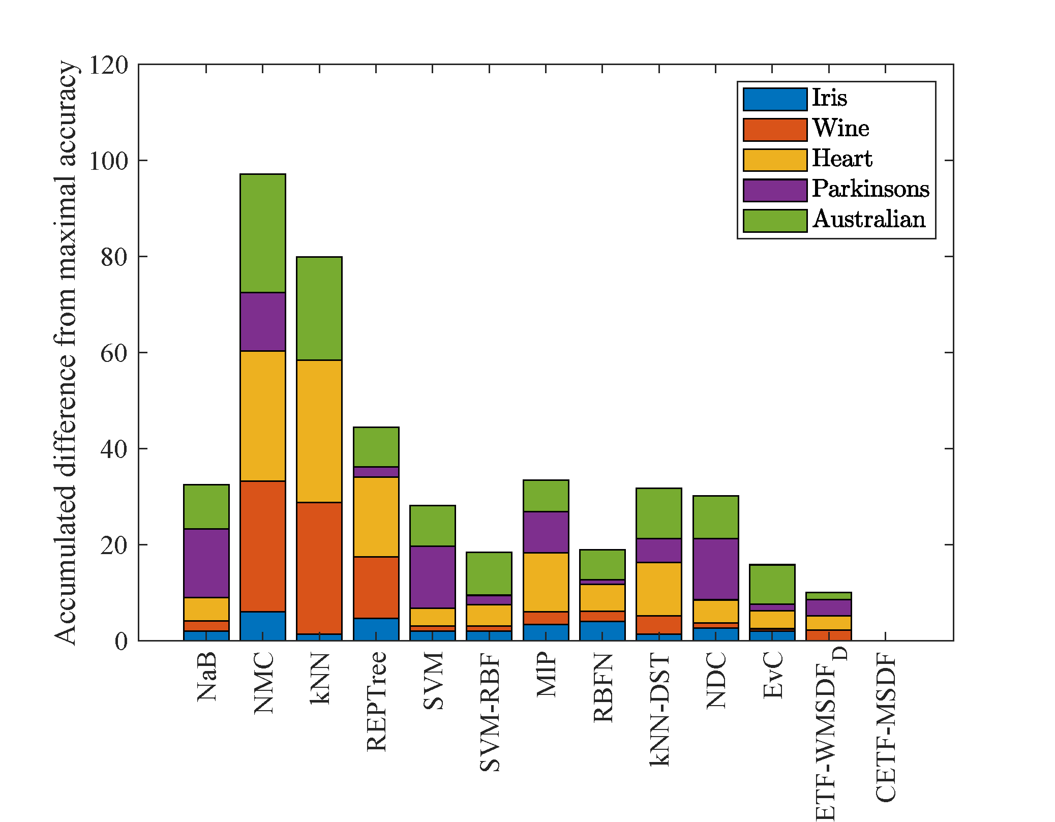
Figure 2 Comparison of accumulated differences from maximal accuracy for different methods.

In addition, the differences between the average classification accuracy of each method and that of the optimal performance are calculated in Table 5. The differences across five datasets are accumulated for further evaluation of their relative performance. As shown in Figure 2, the overall accumulated difference across the five datasets for the CETF-MSDF algorithm is only 0.02%. However, the NaB, NMC, kNN, REPTree, SVM, SVM-RBF, MlP, RBFN, kNN-DST, NDC, EvC and ETF-WMSDF_D algorithms have total accumulated differences of 32.50%, 97.12%, 79.86%, 44.39%, 28.17%, 18.43%, 33.42%, 18.91%, 31.69%, 30.09%, 15.80% and 10.07%, respectively. These results reveal that the superiority of the CETF-MSDF algorithm.

The proposed CETF-MSDF algorithm outperforms other methods because it utilizes CBBA to effectively model and enhance data features through the phase parameter on the occasion of generating CBBAs. To be specific, by fusing appropriate CBBAs expressed by complex numbers, constructive interference will be produced to strengthen modeling data features. Nevertheless, the computational complexity of the CETF-MSDF algorithm is higher comparing with these related methods, which limits its applicability in real-time scenarios. However, in scenarios where accuracy is critical or in certain complex number-based situations, the proposed CETF-MSDF algorithm is the preferred choice. To further improve the processing efficiency of the proposed algorithm for real-time applications, the phase can be modeled in an interpretable manner at an early stage, just like the magnitude.

6. Challenges and open future research directions

In this section, several challenges and open future research directions are summarized and discussed.

6.1 (C)BBA generation with large, heterogeneous and multi-modal data

As science and technology continue to develop, many applications have become heterogeneous sensor-based, so large, heterogeneous and multi-modal data are inevitable [108]. These data have the characteristics of large volume, high variety, but low value. How to generate appropriate BBAs, and even CBBAs, with these large, heterogeneous and multi-modal data to facilitate decisions is a challenging problem in data fusion. It remains an open issue to fuse such heterogeneous and multidimension data.

6.2 Combination of dependent evidence

As discussed in a previous section, DRC in DSET and the CECR in CET require independence among multiple pieces of evidence. However, dependency among some types of data is unavoidable. Several researchers have studied the fusion of dependent evidence from the perspective of combination rule modification and belief structure improvement, but some limitations of these methods restrict their application in data fusion. Therefore, it is necessary to consider how to determine the degree of dependence and how to develop the classical and complex evidence combination rules to fuse dependent evidence.

6.3 Conflict management

In evidence theory, when fusing conflicting data, the classical DRC and CECR may generate counterintuitive results, which impacts the effectiveness of these combination rules in real-world applications of data fusion. In recent decades, the problem of conflict management in the classical DRC has been extensively studied and discussed. Various methods have been proposed, as discussed in Section 3. Careful summary and analysis indicates that no distinct conclusions have been reached. Different applications may require different or even hybrid solutions to manage the conflicting information according to the specific situation, especially for large, heterogeneous and multi-modal data. Furthermore, the current presentation of the CECR in CET requires new strategies to measure and manage conflicts from multisource data modeled in a complex plane.

6.4 Open world

The other limitation of evidence theory is that its FOD must be fully complete. However, in real-world applications, the targets to be detected may be unknown, for example, the detection of unknown diseases, recognition of aircraft types, and classification of unknown elements. Recently, Xiao [109] proposes a generalized quantum evidence theory (GQET) based on a quantum mechanical framework. GQET can facilitate the uncertainty reasoning of data fusion not only in the closed world (when the squared amplitude of the generalized quantum basic belief assignment for the empty set is zero $|\mathds{Q}_{\mathds{M}}(|\emptyset\rangle)|^{2}=0$ , indicating the FOD is complete), but also in the open world (when the squared amplitude of the generalized quantum basic belief assignment for the empty set is nonzero $|\mathds{Q}_{\mathds{M}}(|\emptyset\rangle)|^{2}>0$ , indicating the FOD is incomplete). Particularly, in a closed world, GQET degenerates, called as quantum evidence theory (QET) [109]. In summary, it provides a prospective method to uncertainty representation and reasoning in both of closed and open worlds. Hence, when the FOD is incomplete due to limited knowledge, how to select an appropriate theory, design the combination rule and manage conflicts from multisource data deserve further research and solutions.

6.5 Complexity and real time

In evidence theory, as the number of FODs increases, the power set of the FOD will increase exponentially; how to fuse evidence under an FOD with an abundance of elements remains an open issue. On the other hand, big data has the characteristic of high velocity. The integration of evidence theory for real-time applications requires effective solutions. Our recent work has proposed a novel quantum Dempster's rule of combination, which constructs quantum circuits using quantum logical gates, significantly reducing the computational complexity of Dempster's rule of combination without information loss. This approach offers a promising way to handle such complexity and real-time challenges, making it worthy of further investigation.

7. Conclusion

In this paper, we conducted a comprehensive review of the literature on Dempster–Shafer evidence theory (DSET) for data fusion. We first introduced the basis concepts and knowledge of classical DSET and studied the axioms of Dempster's rule of combination and the characteristics and restraints of DSET. We further provided a review of the classical DSET and its extensions, collectively referred to as classical evidence theory, for data fusion from three aspects, namely, uncertainty modeling, fusion, and decision making. Particularly, in the fusion section, three main kinds of solutions for evidence theory-based data fusion were summarized, including evidential combination rule-based data fusion, evidence pretreatment-based data fusion, and other hybrid evidential conflict models for data fusion, and the typical methods and techniques were described. Next, we studied complex evidence theory for data fusion that benefits from the frame of complex plane modelling in both closed world and open world contexts. Furthermore, we presented classical and complex evidence theory framework-based multisource data fusion algorithms, which were applied to pattern classification. Through comparison with other well-known methods, complex evidence theory framework-based multisource data fusion algorithm showed its superiority to handle pattern classification problem in the complex plane. It also revealed the applicability and limitation of complex evidence theory framework-based multisource data fusion algorithm. On the basis of this survey, analysis and discussion, we present a number of challenges and open issues to help guide future research directions on evidence theory-based data fusion.

Data Availability Statement

Data will be made available on request.

Funding

This work was supported in part by the National Natural Science Foundation of China under Grant 62473067; in part by the Chongqing Talents: Exceptional Young Talents Project under Grant cstc2022ycjh-bgzxm0070; in part by the Chongqing Overseas Scholars Innovation Program under Grant cx2022024.

Conflicts of Interest

The authors declare no conflicts of interest.

Ethical Approval and Consent to Participate

Not applicable.

References

Zhang, L., Xie, Y., Xidao, L., & Zhang, X. (2018, May). Multi-source heterogeneous data fusion. In 2018 International conference on artificial intelligence and big data (ICAIBD) (pp. 47-51). IEEE.
CrossRef Google Scholar
Albahri, A. S., Duhaim, A. M., Fadhel, M. A., Alnoor, A., Baqer, N. S., Alzubaidi, L., ... & Deveci, M. (2023). A systematic review of trustworthy and explainable artificial intelligence in healthcare: Assessment of quality, bias risk, and data fusion. Information Fusion, 96, 156-191.
CrossRef Google Scholar
Lai, J. W., Chang, J., Ang, L. K., & Cheong, K. H. (2020). Multi-level information fusion to alleviate network congestion. Information Fusion, 63, 248-255.
CrossRef Google Scholar
Yager, R. R. (2004). A framework for multi-source data fusion. Information Sciences, 163(1-3), 175-200.
CrossRef Google Scholar
Yang, J. B., Xu, D. L., Xu, X., & Fu, C. (2023). Likelihood analysis of imperfect data. IEEE Transactions on Systems, Man, and Cybernetics: Systems, 53(8), 5046-5057.
CrossRef Google Scholar
Cao, B., Li, C., Song, Y., Qin, Y., & Chen, C. (2022). Network intrusion detection model based on CNN and GRU. Applied Sciences, 12(9), 4184.
CrossRef Google Scholar
Miao, W., Xu, Z., Geng, J., & Jiang, W. (2023). ECAE: Edge-aware class activation enhancement for semisupervised remote sensing image semantic segmentation. IEEE Transactions on Geoscience and Remote Sensing, 61, 1-14.
CrossRef Google Scholar
Judah, A., & Hu, B. (2022). An advanced data fusion method to improve wetland classification using multi-source remotely sensed data. Sensors, 22(22), 8942.
CrossRef Google Scholar
Charte, D., Charte, F., García, S., del Jesus, M. J., & Herrera, F. (2018). A practical tutorial on autoencoders for nonlinear feature fusion: Taxonomy, models, software and guidelines. Information Fusion, 44, 78-96.
CrossRef Google Scholar
Li, T., Song, Y., & Fan, H. (2023). From target tracking to targeting track: A data-driven yet analytical approach to joint target detection and tracking. Signal Processing, 205, 108883.
CrossRef Google Scholar
Deng, X., Xue, S., & Jiang, W. (2023). A novel quantum model of mass function for uncertain information fusion. Information Fusion, 89, 619-631.
CrossRef Google Scholar
Hussain, L. A., Singh, S., Mizouni, R., Otrok, H., & Damiani, E. (2023). A predictive target tracking framework for IoT using CNN–LSTM. Internet of Things, 22, 100744.
CrossRef Google Scholar
Kang, B., & Zhao, C. (2024). Deceptive evidence detection in information fusion of belief functions based on reinforcement learning. Information Fusion, 103, 102102.
CrossRef Google Scholar
Liu, Z., Chen, F., Xu, J., Pei, W., & Lu, G. (2022). Image-text retrieval with cross-modal semantic importance consistency. IEEE Transactions on Circuits and Systems for Video Technology, 33(5), 2465-2476.
CrossRef Google Scholar
Wang, X., Zhu, D., Li, G., Zhang, X. P., & He, Y. (2022). Proposal-Copula-Based Fusion of Spaceborne and Airborne SAR Images for Ship Target Detection⁎⁎. Information Fusion, 77, 247-260.
CrossRef Google Scholar
Chenghai, L. I., Ke, W. A. N. G., Yafei, S. O. N. G., Peng, W. A. N. G., & Lemin, L. I. (2024). Air target intent recognition method combining graphing time series and diffusion models. Chinese Journal of Aeronautics.
CrossRef Google Scholar
Zhang, Y., Wang, X., Jiang, Z., Li, G., & He, Y. (2022). An efficient center-based method with multilevel auxiliary supervision for multiscale SAR ship detection. IEEE Journal of Selected Topics in Applied Earth Observations and Remote Sensing, 15, 7065-7075.
CrossRef Google Scholar
Lau, B. P. L., Marakkalage, S. H., Zhou, Y., Hassan, N. U., Yuen, C., Zhang, M., & Tan, U. X. (2019). A survey of data fusion in smart city applications. Information Fusion, 52, 357-374.
CrossRef Google Scholar
Ding, W., Jing, X., Yan, Z., & Yang, L. T. (2019). A survey on data fusion in internet of things: Towards secure and privacy-preserving fusion. Information Fusion, 51, 129-144.
CrossRef Google Scholar
Deng, X., Jiang, Y., Yang, L. T., Lin, M., Yi, L., & Wang, M. (2019). Data fusion based coverage optimization in heterogeneous sensor networks: A survey. Information Fusion, 52, 90-105.
CrossRef Google Scholar
Ghamisi, P., Rasti, B., Yokoya, N., Wang, Q., Hofle, B., Bruzzone, L., ... & Benediktsson, J. A. (2019). Multisource and multitemporal data fusion in remote sensing: A comprehensive review of the state of the art. IEEE Geoscience and Remote Sensing Magazine, 7(1), 6-39.
CrossRef Google Scholar
Meng, T., Jing, X., Yan, Z., & Pedrycz, W. (2020). A survey on machine learning for data fusion. Information Fusion, 57, 115-129.
CrossRef Google Scholar
El Fissaoui, M., Beni-hssane, A., Ouhmad, S., & El Makkaoui, K. (2021). A survey on mobile agent itinerary planning for information fusion in wireless sensor networks. Archives of computational methods in engineering, 28(3), 1323-1334.
CrossRef Google Scholar
Zhang, Y., Jiang, C., Yue, B., Wan, J., & Guizani, M. (2022). Information fusion for edge intelligence: A survey. Information Fusion, 81, 171-186.
CrossRef Google Scholar
Xinde, L. I., DUNKIN, F., & DEZERT, J. (2023). Multi-source information fusion: Progress and future. Chinese Journal of Aeronautics.
CrossRef Google Scholar
Dempster, A. P. (2008). Upper and lower probabilities induced by a multivalued mapping. In Classic works of the Dempster-Shafer theory of belief functions (pp. 57-72). Berlin, Heidelberg: Springer Berlin Heidelberg.
CrossRef Google Scholar
Shafer, G. et~al. (1976). A mathematical theory of evidence, volume~1. Princeton University Press Princeton.
Google Scholar
Zhang, Z., Ye, S., Zhang, Y., Ding, W., & Wang, H. (2022). Belief combination of classifiers for incomplete data. IEEE/CAA Journal of Automatica Sinica, 9(4), 652-667.
CrossRef Google Scholar
Fujita, H., & Ko, Y. C. (2020). A heuristic representation learning based on evidential memberships: Case study of UCI-SPECTF. International Journal of Approximate Reasoning, 120, 125-137.
CrossRef Google Scholar
Yager, R.~R. and Liu, L. (2008). Classic works of the Dempster--Shafer theory of belief functions, volume 219. Springer.
Google Scholar
Xiong, L., Su, X., & Qian, H. (2021). Conflicting evidence combination from the perspective of networks. Information Sciences, 580, 408-418.
CrossRef Google Scholar
Liu, P., Li, Y., Zhang, X., & Pedrycz, W. (2022). A multiattribute group decision-making method with probabilistic linguistic information based on an adaptive consensus reaching model and evidential reasoning. IEEE Transactions on Cybernetics, 53(3), 1905-1919.
CrossRef Google Scholar
Xu, X., Zheng, J., Yang, J. B., Xu, D. L., & Chen, Y. W. (2017). Data classification using evidence reasoning rule. Knowledge-Based Systems, 116, 144-151.
CrossRef Google Scholar
Tang, S. W., Zhou, Z. J., Hu, C. H., Yang, J. B., & Cao, Y. (2019). Perturbation analysis of evidential reasoning rule. IEEE transactions on systems, man, and cybernetics: systems, 51(8), 4895-4910.
CrossRef Google Scholar
Zhang, B., Zhang, Y., Hu, G., Zhou, Z., Wu, L., & Lv, S. (2020). A method of automatically generating initial parameters for large-scale belief rule base. Knowledge-Based Systems, 199, 105904.
CrossRef Google Scholar
Fu, C., Hou, B., Xue, M., Chang, L., & Liu, W. (2022). Extended belief rule-based system with accurate rule weights and efficient rule activation for diagnosis of thyroid nodules. IEEE Transactions on Systems, Man, and Cybernetics: Systems, 53(1), 251-263.
CrossRef Google Scholar
Zhou, Z. J., Hu, G. Y., Hu, C. H., Wen, C. L., & Chang, L. L. (2019). A survey of belief rule-base expert system. IEEE Transactions on Systems, Man, and Cybernetics: Systems, 51(8), 4944-4958.
CrossRef Google Scholar
Chang, L., Zhang, L., Fu, C., & Chen, Y. W. (2021). Transparent digital twin for output control using belief rule base. IEEE Transactions on cybernetics, 52(10), 10364-10378.
CrossRef Google Scholar
Cao, Y., Zhou, Z., Hu, C., He, W., & Tang, S. (2020). On the interpretability of belief rule-based expert systems. IEEE Transactions on Fuzzy Systems, 29(11), 3489-3503.
CrossRef Google Scholar
Xu, X., Guo, H., Zhang, Z., Shi, P., Huang, W., Li, X., & Brunauer, G. (2024). Fault diagnosis method via one vs rest evidence classifier considering imprecise feature samples. Applied Soft Computing, 161, 111761.
CrossRef Google Scholar
Xu, X., Guo, H., Zhang, Z., Yu, S., Chang, L., Steyskal, F., & Brunauer, G. (2024). A cloud model-based interval-valued evidence fusion method and its application in fault diagnosis. Information Sciences, 658, 119995.
CrossRef Google Scholar
Chen, X., & Deng, Y. (2024). Evidential software risk assessment model on ordered frame of discernment. Expert Systems with Applications, 250, 123786.
CrossRef Google Scholar
Zhou, M., Zheng, Y. Q., Chen, Y. W., Cheng, B. Y., Herrera-Viedma, E., & Wu, J. (2023). A large-scale group consensus reaching approach considering self-confidence with two-tuple linguistic trust/distrust relationship and its application in life cycle sustainability assessment. Information Fusion, 94, 181-199.
CrossRef Google Scholar
Fei, L., Liu, X., & Zhang, C. (2024). An evidential linguistic ELECTRE method for selection of emergency shelter sites. Artificial Intelligence Review, 57(4), 81.
CrossRef Google Scholar
Zadeh, L. A. (1986). A simple view of the Dempster-Shafer theory of evidence and its implication for the rule of combination. AI magazine, 7(2), 85-85.
CrossRef Google Scholar
Smets, P. (2002). The combination of evidence in the transferable belief model. IEEE Transactions on pattern analysis and machine intelligence, 12(5), 447-458.
CrossRef Google Scholar
Dezert, J., & Smarandache, F. (2006). DSmT: A new paradigm shift for information fusion. Infinite Study.
Google Scholar
Deng, Y. (2015). Generalized evidence theory. Applied Intelligence, 43(3), 530-543.
CrossRef Google Scholar
Smarandache, F., Dezert, J., & Tchamova, A. (Eds.). (2023). Advances and Applications of DSmT for Information Fusion (Collected Works. Volume 5).
Google Scholar
Deng, Y. (2022). Random permutation set. International Journal of Computers Communications & Control, 17(1).
CrossRef Google Scholar
Deng, J., Deng, Y., & Yang, J. B. (2024). Random permutation set reasoning. IEEE Transactions on Pattern Analysis and Machine Intelligence.
CrossRef Google Scholar
Deng, X., & Jiang, W. (2023). A framework for the fusion of non-exclusive and incomplete information on the basis of D number theory. Applied Intelligence, 53(10), 11861-11884.
CrossRef Google Scholar
Kouatli, I. (2020). The use of fuzzy logic as augmentation to quantitative analysis to unleash knowledge of participants’ uncertainty when filling a survey: case of cloud computing. IEEE Transactions on Knowledge and Data Engineering, 34(3), 1489-1500.
CrossRef Google Scholar
Akcora, C. G., Gel, Y. R., Kantarcioglu, M., Lyubchich, V., & Thuraisingham, B. (2019). Graphboot: Quantifying uncertainty in node feature learning on large networks. IEEE Transactions on Knowledge and Data Engineering, 33(1), 116-127.
CrossRef Google Scholar
Fei, L., & Wang, Y. (2022). An optimization model for rescuer assignments under an uncertain environment by using Dempster–Shafer theory. Knowledge-Based Systems, 255, 109680.
CrossRef Google Scholar
An, L., Li, M., Boudaren, M. E. Y., & Pieczynski, W. (2018). Unsupervised segmentation of hidden Markov fields corrupted by correlated non-Gaussian noise. International journal of approximate reasoning, 102, 41-59.
CrossRef Google Scholar
Zhang, Z. W., Liu, Z. G., Martin, A., & Zhou, K. (2022). BSC: Belief shift clustering. IEEE Transactions on Systems, Man, and Cybernetics: Systems, 53(3), 1748-1760.
CrossRef Google Scholar
Denoeux, T. (2021). NN-EVCLUS: Neural network-based evidential clustering. Information Sciences, 572, 297-330.
CrossRef Google Scholar
Zhou, K., Martin, A., Pan, Q., & Liu, Z. (2018). SELP: Semi-supervised evidential label propagation algorithm for graph data clustering. International Journal of Approximate Reasoning, 92, 139-154.
CrossRef Google Scholar
He, H., Han, D., & Dezert, J. (2020). Disagreement based semi-supervised learning approaches with belief functions. Knowledge-Based Systems, 193, 105426.
CrossRef Google Scholar
Antoine, V., Guerrero, J. A., & Xie, J. (2021). Fast semi-supervised evidential clustering. International Journal of Approximate Reasoning, 133, 116-132.
CrossRef Google Scholar
Xu, P., Davoine, F., Zha, H., & Denoeux, T. (2016). Evidential calibration of binary SVM classifiers. International Journal of Approximate Reasoning, 72, 55-70.
CrossRef Google Scholar
Denœux, T. (2019). Logistic regression, neural networks and Dempster–Shafer theory: A new perspective. Knowledge-Based Systems, 176, 54-67.
CrossRef Google Scholar
Tong, Z., Xu, P., & Denoeux, T. (2021). An evidential classifier based on Dempster-Shafer theory and deep learning. Neurocomputing, 450, 275-293.
CrossRef Google Scholar
Yager, R. R. (1987). On the Dempster-Shafer framework and new combination rules. Information sciences, 41(2), 93-137.
CrossRef Google Scholar
Dubois, D., & Prade, H. (1988). Representation and combination of uncertainty with belief functions and possibility measures. Computational intelligence, 4(3), 244-264.
CrossRef Google Scholar
Inagaki, T. (2002). Interdependence between safety-control policy and multiple-sensor schemes via Dempster-Shafer theory. IEEE Transactions on Reliability, 40(2), 182-188.
CrossRef Google Scholar
Lefevre, E., Colot, O., & Vannoorenberghe, P. (2002). Belief function combination and conflict management. Information fusion, 3(2), 149-162.
CrossRef Google Scholar
Zhang, L. (1994). Representation, independence, and combination of evidence in the Dempster-Shafer theory. In Advances in the Dempster-Shafer theory of evidence (pp. 51-69). https://dl.acm.org/doi/abs/10.5555/186965.186968
Google Scholar
Mahler, R. P. (1996). Combining ambiguous evidence with respect to ambiguous a priori knowledge. I. Boolean logic. IEEE Transactions on Systems, Man, and Cybernetics-Part A: Systems and Humans, 26(1), 27-41.
CrossRef Google Scholar
Jiang, W., & Zhan, J. (2017). A modified combination rule in generalized evidence theory. Applied Intelligence, 46(3), 630-640.
CrossRef Google Scholar
Xiao, F. (2020). Generalization of Dempster–Shafer theory: A complex mass function. Applied Intelligence, 50(10), 3266-3275.
CrossRef Google Scholar
Xiao, F. (2020). Generalized belief function in complex evidence theory. Journal of Intelligent & Fuzzy Systems, 38(4), 3665-3673.
CrossRef Google Scholar
Chen, X., & Deng, Y. (2023). A novel combination rule for conflict management in data fusion. Soft Computing, 27(22), 16483-16492.
CrossRef Google Scholar
Jousselme, A. L., Grenier, D., & Bossé, É. (2001). A new distance between two bodies of evidence. Information fusion, 2(2), 91-101.
CrossRef Google Scholar
Jousselme, A. L., & Maupin, P. (2012). Distances in evidence theory: Comprehensive survey and generalizations. International Journal of Approximate Reasoning, 53(2), 118-145.
CrossRef Google Scholar
Han, D., Dezert, J., & Yang, Y. (2016). Belief interval-based distance measures in the theory of belief functions. IEEE Transactions on Systems, Man, and Cybernetics: Systems, 48(6), 833-850.
CrossRef Google Scholar
Smets, P., & Kennes, R. (1994). The transferable belief model. Artificial intelligence, 66(2), 191-234.
CrossRef Google Scholar
Liu, W. (2006). Analyzing the degree of conflict among belief functions. Artificial intelligence, 170(11), 909-924.
CrossRef Google Scholar
Jiang, W. (2018). A correlation coefficient for belief functions. International Journal of Approximate Reasoning, 103, 94-106.
CrossRef Google Scholar
Deng, Y. (2020). Uncertainty measure in evidence theory. Science China Information Sciences, 63(11), 210201.
CrossRef Google Scholar
Abellán, J. (2017). Analyzing properties of Deng entropy in the theory of evidence. Chaos, Solitons & Fractals, 95, 195-199.
CrossRef Google Scholar
Deng, Y. (2020). Information volume of mass function. International Journal of Computers Communications & Control, 15(6).
Google Scholar
Liao, H., Ren, Z., & Fang, R. (2020). A Deng-entropy-based evidential reasoning approach for multi-expert multi-criterion decision-making with uncertainty. International Journal of Computational Intelligence Systems, 13(1), 1281-1294.
CrossRef Google Scholar
Zhao, T., Li, Z., & Deng, Y. (2024). Linearity in Deng entropy. Chaos, Solitons & Fractals, 178, 114388.
CrossRef Google Scholar
Cui, Y., & Deng, X. (2023). Plausibility entropy: A new total uncertainty measure in evidence theory based on plausibility function. IEEE Transactions on Systems, Man, and Cybernetics: Systems, 53(6), 3833-3844.
CrossRef Google Scholar
Qiang, C., Deng, Y., & Cheong, K. H. (2022). Information fractal dimension of mass function. Fractals, 30(06), 2250110.
CrossRef Google Scholar
Zhu, L., Zhou, Q., Deng, Y., & Cheong, K. H. (2024). Fractal-based basic probability assignment: A transient mass function. Information Sciences, 652, 119767.
CrossRef Google Scholar
Li, D., Deng, Y., & Cheong, K. H. (2021). Multisource basic probability assignment fusion based on information quality. International Journal of Intelligent Systems, 36(4), 1851-1875.
CrossRef Google Scholar
Daniel, M. (2010, June). Conflicts within and between belief functions. In International Conference on Information Processing and Management of Uncertainty in Knowledge-Based Systems (pp. 696-705). Berlin, Heidelberg: Springer Berlin Heidelberg.
CrossRef Google Scholar
Lefevre, E., & Elouedi, Z. (2013). How to preserve the conflict as an alarm in the combination of belief functions?. Decision Support Systems, 56, 326-333.
CrossRef Google Scholar
Abellán, J., & Bossé, É. (2016). Drawbacks of uncertainty measures based on the pignistic transformation. IEEE Transactions on Systems, Man, and Cybernetics: Systems, 48(3), 382-388.
CrossRef Google Scholar
Martin, L., & Sudano, J. J. (2006, July). Yet another paradigm illustrating evidence fusion (YAPIEF). In 2006 9th international conference on information fusion (pp. 1-7). IEEE.
CrossRef Google Scholar
Cuzzolin, F. (2007). Two new Bayesian approximations of belief functions based on convex geometry. IEEE Transactions on Systems, Man, and Cybernetics, Part B (Cybernetics), 37(4), 993-1008.
CrossRef Google Scholar
Han, D., Dezert, J., & Duan, Z. (2015). Evaluation of probability transformations of belief functions for decision making. IEEE Transactions on Systems, Man, and Cybernetics: Systems, 46(1), 93-108.
CrossRef Google Scholar
Liu, Z. G., Fu, Y. M., Pan, Q., & Zhang, Z. W. (2022). Orientational distribution learning with hierarchical spatial attention for open set recognition. IEEE Transactions on Pattern Analysis and Machine Intelligence, 45(7), 8757-8772.
CrossRef Google Scholar
Liu, Z. G., Qiu, G. H., Wang, S. Y., Li, T. C., & Pan, Q. (2021). A new belief-based bidirectional transfer classification method. IEEE Transactions on Cybernetics, 52(8), 8101-8113.
CrossRef Google Scholar
Xiao, F., & Pedrycz, W. (2022). Negation of the quantum mass function for multisource quantum information fusion with its application to pattern classification. IEEE Transactions on Pattern Analysis and Machine Intelligence, 45(2), 2054-2070.
CrossRef Google Scholar
Hu, B. G. (2013). What are the differences between Bayesian classifiers and mutual-information classifiers?. IEEE transactions on neural networks and learning systems, 25(2), 249-264.
CrossRef Google Scholar
Veenman, C. J., & Reinders, M. J. (2005). The nearest subclass classifier: A compromise between the nearest mean and nearest neighbor classifier. IEEE Transactions on Pattern Analysis and Machine Intelligence, 27(9), 1417-1429.
CrossRef Google Scholar
Cover, T., & Hart, P. (1967). Nearest neighbor pattern classification. IEEE transactions on information theory, 13(1), 21-27.
CrossRef Google Scholar
Freund, Y., & Mason, L. (1999, June). The alternating decision tree learning algorithm. In icml (Vol. 99, pp. 124-133).
Google Scholar
Chang, C. C., & Lin, C. J. (2011). LIBSVM: A library for support vector machines. ACM transactions on intelligent systems and technology (TIST), 2(3), 1-27.
CrossRef Google Scholar
Castro, C. L., & Braga, A. P. (2013). Novel cost-sensitive approach to improve the multilayer perceptron performance on imbalanced data. IEEE transactions on neural networks and learning systems, 24(6), 888-899.
CrossRef Google Scholar
CHEN S, G. M., & Grant, P. M. (1991). Orthogonal Least Squares Learning Algorithm for Radial Basis Function Networks. IEEE Transactions on Neural Networks, 2(2), 302-309.
CrossRef Google Scholar
Denoeux, T. (1995). A k-nearest neighbor classification rule based on Dempster-Shafer theory. IEEE transactions on systems, man, and cybernetics, 25(5), 804-813.
CrossRef Google Scholar
Xu, P., Deng, Y., Su, X., & Mahadevan, S. (2013). A new method to determine basic probability assignment from training data. Knowledge-Based Systems, 46, 69-80.
CrossRef Google Scholar
Wang, Y. M., Pan, X. H., He, S. F., Dutta, B., García-Zamora, D., & Martínez, L. (2022). A new decision-making framework for site selection of electric vehicle charging station with heterogeneous information and multigranular linguistic terms. IEEE Transactions on Fuzzy Systems, 31(2), 485-499.
CrossRef Google Scholar
Xiao, F. (2023). Generalized quantum evidence theory. Applied Intelligence, 53(11), 14329-14344.
CrossRef Google Scholar

Cite This Article

APA Style

Xiao, F., Wen, J., Pedrycz, W., & Aritsugi, M. (2024). Complex Evidence Theory for Multisource Data Fusion. Chinese Journal of Information Fusion, 1(2), 134–159. https://doi.org/10.62762/CJIF.2024.999646

Export Citation

RIS Format

Compatible with EndNote, Zotero, Mendeley, and other reference managers

RIS format data for reference managers

TY  - JOUR
AU  - Xiao, Fuyuan
AU  - Wen, Junhao
AU  - Pedrycz, Witold
AU  - Aritsugi, Masayoshi
PY  - 2024
DA  - 2024/09/30
TI  - Complex Evidence Theory for Multisource Data Fusion
JO  - Chinese Journal of Information Fusion
T2  - Chinese Journal of Information Fusion
JF  - Chinese Journal of Information Fusion
VL  - 1
IS  - 2
SP  - 134
EP  - 159
DO  - 10.62762/CJIF.2024.999646
UR  - https://www.icck.org/article/abs/CJIF.2024.999646
KW  - multisource data fusion
KW  - Dempster-Shafer evidence theory
KW  - complex evidence theory
KW  - quantum evidence theory
KW  - uncertainty modeling
KW  - conflict management
KW  - belief function
KW  - decision making
KW  - pattern classification
AB  - Data fusion is a prevalent technique for assembling imperfect raw data coming from multiple sources to capture reliable and accurate information. Dempster–Shafer evidence theory is one of useful methodologies in the fusion of uncertain multisource information. The existing literature lacks a thorough and comprehensive review of the recent advances of Dempster– Shafer evidence theory for data fusion. Therefore, the state of the art has to be surveyed to gain insight into how Dempster–Shafer evidence theory is beneficial for data fusion and how it evolved over time. In this paper, we first provide a comprehensive review of data fusion methods based on Dempster–Shafer evidence theory and its extensions, collectively referred to as classical evidence theory, from three aspects of uncertainty modeling, fusion, and decision making. Next, we study and explore complex evidence theory for data fusion in both closed world and open world contexts that benefits from the frame of complex plane modelling. We then present classical and complex evidence theory framework-based multisource data fusion algorithms, which are applied to pattern classification to compare and demonstrate their applicabilities. The research results indicate that the complex evidence theory framework can enhance the capabilities of uncertainty modeling and reasoning by generating constructive interference through the fusion of appropriate complex basic belief assignment functions modeled by complex numbers. Through analysis and comparison, we finally propose several challenges and identify open future research directions in evidence theorybased data fusion.
SN  - 2998-3371
PB  - Institute of Central Computation and Knowledge
LA  - English
ER  -

BibTeX Format

Compatible with LaTeX, BibTeX, and other reference managers

BibTeX format data for LaTeX and reference managers

@article{Xiao2024Complex,
  author = {Fuyuan Xiao and Junhao Wen and Witold Pedrycz and Masayoshi Aritsugi},
  title = {Complex Evidence Theory for Multisource Data Fusion},
  journal = {Chinese Journal of Information Fusion},
  year = {2024},
  volume = {1},
  number = {2},
  pages = {134-159},
  doi = {10.62762/CJIF.2024.999646},
  url = {https://www.icck.org/article/abs/CJIF.2024.999646},
  abstract = {Data fusion is a prevalent technique for assembling imperfect raw data coming from multiple sources to capture reliable and accurate information. Dempster–Shafer evidence theory is one of useful methodologies in the fusion of uncertain multisource information. The existing literature lacks a thorough and comprehensive review of the recent advances of Dempster– Shafer evidence theory for data fusion. Therefore, the state of the art has to be surveyed to gain insight into how Dempster–Shafer evidence theory is beneficial for data fusion and how it evolved over time. In this paper, we first provide a comprehensive review of data fusion methods based on Dempster–Shafer evidence theory and its extensions, collectively referred to as classical evidence theory, from three aspects of uncertainty modeling, fusion, and decision making. Next, we study and explore complex evidence theory for data fusion in both closed world and open world contexts that benefits from the frame of complex plane modelling. We then present classical and complex evidence theory framework-based multisource data fusion algorithms, which are applied to pattern classification to compare and demonstrate their applicabilities. The research results indicate that the complex evidence theory framework can enhance the capabilities of uncertainty modeling and reasoning by generating constructive interference through the fusion of appropriate complex basic belief assignment functions modeled by complex numbers. Through analysis and comparison, we finally propose several challenges and identify open future research directions in evidence theorybased data fusion.},
  keywords = {multisource data fusion, Dempster-Shafer evidence theory, complex evidence theory, quantum evidence theory, uncertainty modeling, conflict management, belief function, decision making, pattern classification},
  issn = {2998-3371},
  publisher = {Institute of Central Computation and Knowledge}
}

Article Metrics

Citations:

Google Scholar

Crossref

Scopus

Web of Science

Article Access Statistics:

PDF Downloads: 1835

Publisher's Note

ICCK stays neutral with regard to jurisdictional claims in published maps and institutional affiliations.

Rights and Permissions

This article is an open access article distributed under the terms and conditions of the Creative Commons Attribution (CC BY) license.