Modified Hiemenz Stagnation Point Flow of Second Grade Nano Fluid

Aamar Kamal Abbasi; Ali B. M. Ali; Misbah Naseer; Waseh Farooq; Shahid Ali; Muhammad Rafiq

doi:10.62762/JAM.2025.411313

Abstract

Three-dimensional (3D) flow of a viscoelastic fluid in the neighborhood of new family of modified stagnation point depending on shear to strain ratio over a flat surface is numerically investigated. Similarity equations are obtained from the fundamental conservation laws of mass, momentum, energy and nanoparticle concentration. The resulting set of nonlinear equations are solved numerically using an implicit finite difference scheme known as Keller-Box Method. A comparative analysis for modified Hiemenz flow, non-axisymmetric stagnation point and axisymmetric stagnation point flow is carried out. Velocity, temperature and concentration profiles, skin frictions local Nusselt and Sherwood numbers are graphically presented and their variation with involved parameters is discussed in detail. We found that velocity concentration and temperature profiles increase by an increasing the values of We.

Graphical Abstract

Modified Hiemenz Stagnation Point Flow of Second Grade Nano Fluid

Click image to view fullscreen

Keywords

modified hiemenz flow second grade fluid numerical solution nanofluid Keller-Box method

1. Introduction

Stagnation point flows with varied concrete outcomes in industry and having ample applications in friction reduction and transpiration cooling the cooling of a nuclear reactor, phenomena of drag reduction, radial diffusers, and thrust bearings, several theoretical investigations have been reported by many researchers. Hiemenz [1] first addressed two dimensional flow of Newtonian fluid in the stagnation region over a flat plate. The same problem was discussed by Homann [11] for axisymmetric stagnation point flow on a smooth sheet. Lin et al. [17] perform a theoretical analysis to discuss the effects of slip on boundary layer flow of incompressible viscous fluid in the neighborhood of the stagnation point on the flat plate. Rott [22] analyzed two-dimensional, unstable, sticky, incompressible flow in the vicinity of a stagnation point over a plate. Libby [16] presented the study of boundary-layer over an axi-symmetric stagnation point flow. Gorla [8] investigated that the properties of fluid dynamics of an axisymmetric stagnation point flow on a moving cylinder. Weidman et al. [31] investigated the viscous fluid motion generated by axisymmetric stagnation-point flow in a porous medium. Takhar et al. [28] investigated the flow when both the free stream velocity and velocity of the cylinder vary arbitrarily with time, the unsteady viscous flow in the vicinity of an axisymmetric stagnation point of an infinite circular cylinder. Ziabakhsh et al. [34] used a new analytical technique called the homotopy analysis method (HAM), the non-linear Brinkman equation for the stagnation-point flow in a porous medium is analytically solved. The numerical solution (NS) is compared with the analytical results, and the comparison shows that there is good agreement between the NS and HAM solution. Weidman [30] investigated the impingement of two axisymmetric stagnation-point flows on a spinning, radially extending disc which are classical Homann stagnation point flow and circular Argawal stagnation flow. A disk surface velocity is obtained in the form of logarithmic spiral by the combined effect of linear radial stretching and uniform rotation. Sajid et al. [25] studied the axisymmetric stagnation point flow of viscous fluid over lubricant surface. Santra et al. [27] analyzed the axisymmetric stagnation point flow of viscous fluid and a thin non-Newtonian liquid coating of variable thickness lubricates a flat surface against which a Newtonian fluid impinges orthogonally. Ishihara et al. [12] consider the axisymmetric stagnation point flow of one fluid impinging on a disk covered with a second fluid. A similarity reduction is employed to reduce the governing PDEs to a nonlinear ODE boundary value problem. Zhong et al. [33] investigated the axisymmetric stagnation flow of an incompressible viscous fluid on a body moving with the oncoming flow at a time-dependent velocity.

The phenomenon of heat transfer is widely used in industrial and biomedical applications, including the cooling of electronic equipment, the cooling of nuclear reactors, the production of electricity, the conduction of heat through tissues, and many more. Wang [29] observed some forced convection cooling processes a coolant is impinged on a continuously moving plate and discussed the fluid dynamics and heat transmission near the stagnation point. Conduction of heat with constant suction, injection and Homann hydro magnetic flow has been examined by Attia [5]. Saleh et al. [26] investigated the axial velocity and uniform normal transpiration in a moving pipe, together with the viscous flow and conduction of heat around an axisymmetric stagnation point flow. The impinging unbounded stream has an unvarying strain rate and is steady. In this problem, the Navier-Stokes equations and the energy equation have an exact solution. Also when the cylinder's axial velocity and its temperature of its wall flow fluctuate which defined functions that depends upon time, the general self-similar solution is achieved. Rahimi [21] examined the time dependent viscous flow and heat transfer around an axi-symmetric stagnation point flow on a tube with changing degree of velocities. Mahabaleshwar et al. [18] investigated the time dependent flow of a Newtonian fluids via a stagnation point caused by a straight surface with mass transpiration, the effects of magneto hydro dynamic (MHD) and thermal radiation are taken into consideration. Theoretically, they discussed the properties of heat impinging on the surface.

Flows of Non-Newtonian fluids have been investigated by the several researchers under various conditions because of their occurrence in the engineering and industrial processes. Such fluids are specifically quite common in the process of manufacturing coated sheets, foods, optical fibers, drilling muds, plastic polymers, etc. It is well known that all the non-Newtonian fluids cannot be described by a single constitutive relationship in view of their diverse characteristics.

Hence several models of non-Newtonian fluids have been suggested. The non-Newtonian fluids have been mainly classified into three types which are called the differential, the rate and the integral. Out of these, the differential type fluids have been attracted much by the researchers. A simplest subclass of differential type model is called a second-grade fluid.

Barış et al. [6] solved the steady three-dimensional flow of a second grade fluid near the stagnation point flow over an infinite plate. The plate is moving parallel to itself with uniform velocity. Nawaz et al. [20] discussed the second grade fluid with magnetohydrodynamics stagnation point flow and heat transfer over a radially stretching sheet. Moreover, the flow problems are analyzed with Newtonian heating, Soret and Dofour effects. Ahmad et al. [10] solved the problem of axisymmetric stagnation-point flow of second grade fluid over a lubricated surface in the presence of heat transfer. The lubricant assumed to have a thin layer of variable thickness which allows a partial slip over the surface and obeys the constitutive relationship of a power law fluid. Hayat et al. [9] presented the second-grade fluid's magnetohydrodynamic (MHD) stagnation point flow over a stretching cylinder in this study with heat and mass transfer. Also they investigated the effects of Joule heating and viscous dissipation. Saif et al. [24] examined the flow of second-grade nanomaterial towards a nonlinear stretching surface with varying surface thickness. The melting heat and mixed convection effects are used to investigate the heat transfer process in the presence of Brownian motion and thermophoresis effects. Ariel [3] discussed the time independent axisymmetric laminar flow of second grade fluid on a radially stretching surface. Ariel [4] investigated the stagnation point flow of second grade fluid in two dimension. A boundary value problem that has differential equations of order one more than there are possible boundary conditions governs the flow. Ariel [2] analyzed the numerical algorithm of laminar two-dimensional flow of a second grade fluid near a stagnation point and the flow of second grade fluid over a stretching surface in the presence of porous medium. Labropulu et al. [15] considered the constant two-dimensional stagnation-point flow of a fluid with slip condition. Sahoo et al. [23] studied an incompressible, electrically conducting, non-Newtonian second-grade fluid impinging on a flat plate of constant axisymmetric flow and heat transfer.

To get the best thermal characteristics for nanoparticles with uniform dispersion and stable suspension in a base fluid, nano fluids are crucial. Due to their significance, nano fluids are frequently used in many engineering and industrial projects. They are also utilized in microelectronics, heat exchangers, nuclear reactors, space technology, the plastics industry, biomedical technology and ships. Nadeem et al. [19] noticed that the axisymmetric flow of a second-grade nanofluid with varying viscosity in the neighborhood of stagnation point in the presence of Cattaneo-Christov double diffusion model. An electrically conducting nanofluid's unsteady 3D non-axisymmetric Homann flow is investigated when buoyant forces are present by Khan et al. [13]. Khan et al. [14] analyzed the non-axisymmetric Homann stagnation-point flow of Walter's B nanofluid in the occurrence of a time-independent free stream is taken into account, together with magneto hydro dynamic (MHD) and non-linear Rosseland thermal radiation. Additionally, Buongiorno's model analyses the important effects of motion.

2. Flow Model

Three dimensional modified Hiemenz flow of viscoelastic fluid over a flat plate is conceded. The Buongiorno's nano fluid model is used to intricate the impacts of thermophoresis and Brownian motion. The Cartesian coordinate system $(x,y,z)$ is taken in such a way $z=0$ represents the surface of the plate maintained at constant temperature $T_{w}$ and constant concentration $C_{w}$ the fluid occupied the space $z>0$ and the rheology of the fluid is specified by the stress tensor $\tau=-PI+\mu A_{1}+\alpha_{1}A_{2}+\alpha_{2}A_{1}^{2}$ with the thermodynamic constrants $\mu\geq 0,$ in which $P$ represents the pressure $A_{1}$ and $A_{2}$ are kinematic tensors $\alpha_{1}$ and $\alpha_{2}$ represents the normal stress moduli.

A detail discussion on the restriction on these parameters is available in the literature we follow Dunn et al. [7] and we used $\mu\geq 0,\alpha_{1}\geq 0$ and $\alpha_{1}+\alpha_{2}=0$ thermodynamic conditions in the sub sequential analysis. In the absence of body forces the governing equations utilizing conservation laws of mas, momentum, energy, nanoparticle concentration and convective diffusion equation are In the potential region velocity components are $u=\lambda_{1}x,v=\lambda_{2}y,z=-az$ . The equations governing the present flow are:

\frac{\partial u}{\partial x}+\frac{\partial v}{\partial y}+\frac{\partial w}{% \partial z}=0,

X-component:

\begin{split}\rho\biggl{[}u\frac{\partial u}{\partial x}&+v\frac{\partial u}{% \partial y}+w\frac{\partial u}{\partial z}\biggr{]}\\ &=-\frac{\partial p}{\partial x}\\ &+\mu\left[2\frac{\partial^{2}u}{\partial x^{2}}+\frac{\partial^{2}u}{\partial y% ^{2}}+\frac{\partial^{2}v}{\partial x\partial y}+\frac{\partial^{2}u}{\partial z% ^{2}}+\frac{\partial^{2}w}{\partial x\partial z}\right]\\ &+\end{split}

\alpha_{1}\left[\begin{aligned} &2u\frac{\partial^{3}u}{\partial x^{3}}+2\frac% {\partial u}{\partial x}\frac{\partial^{2}u}{\partial x^{2}}+2\frac{\partial v% }{\partial x}\frac{\partial^{2}u}{\partial x\partial y}+2v\frac{\partial^{3}u}% {\partial x^{2}\partial y}+2\frac{\partial w}{\partial x}\frac{\partial^{2}u}{% \partial x\partial z}+2w\frac{\partial^{3}u}{\partial x^{2}\partial z}+2\frac{% \partial v}{\partial x}\frac{\partial^{2}v}{\partial x^{2}}\\ &-2\frac{\partial u}{\partial y}\frac{\partial^{2}u}{\partial x\partial y}-2% \frac{\partial u}{\partial z}\frac{\partial^{2}u}{\partial x\partial z}+\frac{% \partial u}{\partial y}\frac{\partial^{2}u}{\partial x\partial y}+u\frac{% \partial^{3}u}{\partial y^{2}\partial x}+\frac{\partial u}{\partial y}\frac{% \partial^{2}v}{\partial x^{2}}+u\frac{\partial^{3}v}{\partial x^{2}\partial y}% +\frac{\partial v}{\partial y}\frac{\partial^{2}u}{\partial y^{2}}\\ &+\frac{\partial v}{\partial y}\frac{\partial^{2}v}{\partial x\partial y}+v% \frac{\partial^{3}v}{\partial x\partial y^{2}}+\frac{\partial w}{\partial y}% \frac{\partial^{2}u}{\partial y\partial z}+w\frac{\partial^{3}u}{\partial y^{2% }\partial z}+\frac{\partial w}{\partial y}\frac{\partial^{2}v}{\partial x% \partial z}+w\frac{\partial^{3}v}{\partial x\partial y\partial z}+\frac{% \partial u}{\partial y}\frac{\partial^{2}u}{\partial x\partial y}\\ &-\frac{\partial v}{\partial y}\frac{\partial^{2}u}{\partial y^{2}}-\frac{% \partial u}{\partial y}\frac{\partial^{2}v}{\partial y^{2}}+\frac{\partial v}{% \partial y}\frac{\partial^{2}v}{\partial y\partial x}+\frac{\partial v}{% \partial x}\frac{\partial^{2}v}{\partial y^{2}}-\frac{\partial v}{\partial x}% \frac{\partial^{2}u}{\partial x\partial y}-\frac{\partial u}{\partial x}\frac{% \partial^{2}v}{\partial x\partial y}+\frac{\partial w}{\partial y}\frac{% \partial^{2}w}{\partial x\partial y}+\frac{\partial w}{\partial x}\frac{% \partial^{2}w}{\partial y^{2}}\\ &-\frac{\partial v}{\partial z}\frac{\partial^{2}u}{\partial z\partial y}-% \frac{\partial u}{\partial z}\frac{\partial^{2}v}{\partial y\partial z}+\frac{% \partial u}{\partial z}\frac{\partial^{2}u}{\partial x\partial z}+u\frac{% \partial^{3}u}{\partial x\partial z^{2}}+\frac{\partial u}{\partial z}\frac{% \partial^{2}w}{\partial x^{2}}+u\frac{\partial^{3}w}{\partial x^{2}\partial z}% +\frac{\partial v}{\partial z}\frac{\partial^{2}u}{\partial y\partial z}\\ &+\frac{\partial v}{\partial z}\frac{\partial^{2}w}{\partial x\partial y}+v% \frac{\partial^{3}w}{\partial x\partial y\partial z}+\frac{\partial w}{% \partial z}\frac{\partial^{2}u}{\partial z^{2}}+w\frac{\partial^{3}u}{\partial z% ^{3}}+\frac{\partial w}{\partial z}\frac{\partial^{2}w}{\partial x\partial z}+% w\frac{\partial^{3}w}{\partial x\partial z^{2}}+\frac{\partial u}{\partial z}% \frac{\partial^{2}u}{\partial x\partial z}\\ &+\frac{\partial v}{\partial z}\frac{\partial^{2}v}{\partial x\partial z}+% \frac{\partial v}{\partial x}\frac{\partial^{2}v}{\partial z^{2}}+\frac{% \partial w}{\partial z}\left(\frac{\partial^{2}w}{\partial x\partial z}-\frac{% \partial^{2}u}{\partial z^{2}}\right)+\frac{\partial w}{\partial x}\left(\frac% {\partial^{2}u}{\partial x\partial z}-\frac{\partial^{2}u}{\partial x\partial z% }\right)-\frac{\partial u}{\partial x}\frac{\partial^{2}w}{\partial x\partial z% }-\frac{\partial u}{\partial z}\frac{\partial^{2}w}{\partial z^{2}}\\ &+2\frac{\partial w}{\partial x}\frac{\partial^{2}w}{\partial x^{2}}+v\frac{% \partial^{3}u}{\partial y^{3}}+\frac{\partial u}{\partial x}\frac{\partial^{2}% u}{\partial y^{2}}-\frac{\partial w}{\partial y}\frac{\partial^{2}u}{\partial y% \partial z}-\frac{\partial u}{\partial y}\frac{\partial^{2}w}{\partial y% \partial z}+v\frac{\partial^{3}u}{\partial y\partial z^{2}}+\frac{\partial u}{% \partial x}\frac{\partial^{2}u}{\partial z^{2}}\end{aligned}\right],

Y-component:

\begin{split}&\rho\left[u\frac{\partial v}{\partial x}+v\frac{\partial v}{% \partial y}+w\frac{\partial v}{\partial z}\right]=-\frac{\partial p}{\partial y% }+\mu\left[2\frac{\partial^{2}v}{\partial y^{2}}+\frac{\partial^{2}u}{\partial x% \partial y}+\frac{\partial^{2}v}{\partial x^{2}}+\frac{\partial^{2}w}{\partial y% \partial z}+\frac{\partial^{2}v}{\partial z^{2}}\right]\\ &+\alpha_{1}\left[\begin{aligned} &\frac{\partial u}{\partial x}\frac{\partial% ^{2}u}{\partial x\partial y}+u\frac{\partial^{3}u}{\partial x^{2}\partial y}+% \frac{\partial u}{\partial x}\frac{\partial^{2}v}{\partial x^{2}}+u\frac{% \partial^{3}v}{\partial x^{3}}+\frac{\partial v}{\partial x}\frac{\partial^{2}% u}{\partial y^{2}}+v\frac{\partial^{3}u}{\partial y^{2}\partial x}+\frac{% \partial v}{\partial x}\frac{\partial^{2}v}{\partial x\partial y}\\ &+v\frac{\partial^{3}v}{\partial x^{2}\partial y}+\frac{\partial w}{\partial x% }\frac{\partial^{2}u}{\partial y\partial z}+w\frac{\partial^{3}u}{\partial x% \partial y\partial z}+\frac{\partial w}{\partial x}\frac{\partial^{2}v}{% \partial x\partial z}+w\frac{\partial^{3}v}{\partial x^{2}\partial z}+\frac{% \partial u}{\partial y}\frac{\partial^{2}u}{\partial x^{2}}+\frac{\partial u}{% \partial x}\frac{\partial^{2}u}{\partial x\partial y}\\ &-\frac{\partial v}{\partial x}\frac{\partial^{2}u}{\partial x\partial y}-% \frac{\partial u}{\partial y}\frac{\partial^{2}v}{\partial x\partial y}+\frac{% \partial v}{\partial y}\frac{\partial^{2}v}{\partial x^{2}}+\frac{\partial v}{% \partial x}\frac{\partial^{2}v}{\partial x\partial y}-\frac{\partial v}{% \partial x}\frac{\partial^{2}u}{\partial x^{2}}-\frac{\partial u}{\partial x}% \frac{\partial^{2}v}{\partial x^{2}}+\frac{\partial w}{\partial x}\frac{% \partial^{2}w}{\partial x\partial y}\\ &+\frac{\partial w}{\partial y}\frac{\partial^{2}w}{\partial x^{2}}-\frac{% \partial v}{\partial z}\frac{\partial^{2}u}{\partial x\partial z}-\frac{% \partial u}{\partial z}\frac{\partial^{2}v}{\partial x\partial z}+2\frac{% \partial u}{\partial y}\frac{\partial^{2}v}{\partial x\partial z}+2u\frac{% \partial^{3}v}{\partial y^{2}\partial x}+\frac{\partial u}{\partial z}\frac{% \partial^{2}v}{\partial x\partial z}\\ &+u\frac{\partial^{3}v}{\partial z^{2}\partial x}+\frac{\partial u}{\partial z% }\frac{\partial^{2}w}{\partial x\partial y}+u\frac{\partial^{3}w}{\partial x% \partial y\partial z}+\frac{\partial v}{\partial z}\frac{\partial^{2}v}{% \partial y\partial z}+v\frac{\partial^{3}v}{\partial z^{2}\partial x}+\frac{% \partial v}{\partial z}\frac{\partial^{2}w}{\partial y^{2}}+v\frac{\partial^{3% }w}{\partial y^{2}\partial z}\\ &+\frac{\partial w}{\partial z}\frac{\partial^{2}v}{\partial z^{2}}+w\frac{% \partial^{3}v}{\partial z^{3}}+\frac{\partial w}{\partial z}\frac{\partial^{2}% w}{\partial y\partial z}+w\frac{\partial^{3}w}{\partial z^{2}\partial y}+\frac% {\partial u}{\partial y}\frac{\partial^{2}u}{\partial z^{2}}+\frac{\partial u}% {\partial z}\frac{\partial^{2}u}{\partial y\partial z}+\frac{\partial v}{% \partial z}\frac{\partial^{2}v}{\partial y\partial z}\\ &+\frac{\partial v}{\partial y}\frac{\partial^{2}v}{\partial z^{2}}+\frac{% \partial w}{\partial z}\frac{\partial^{2}w}{\partial y\partial z}+\frac{% \partial w}{\partial y}\frac{\partial^{2}w}{\partial z^{2}}-\frac{\partial w}{% \partial x}\frac{\partial^{2}v}{\partial x\partial z}-\frac{\partial v}{% \partial x}\frac{\partial^{2}w}{\partial x\partial z}-\frac{\partial w}{% \partial y}\frac{\partial^{2}v}{\partial y\partial z}-\frac{\partial v}{% \partial y}\frac{\partial^{2}w}{\partial y\partial z}\\ &-\frac{\partial w}{\partial z}\frac{\partial^{2}v}{\partial z^{2}}-\frac{% \partial v}{\partial z}\frac{\partial^{2}w}{\partial z^{2}}+2v\frac{\partial^{% 3}v}{\partial y^{3}}+2\frac{\partial u}{\partial y}\frac{\partial^{2}v}{% \partial y^{2}}+2w\frac{\partial^{3}v}{\partial y^{2}\partial z}+2\frac{% \partial w}{\partial y}\frac{\partial^{2}v}{\partial y\partial z}+2\frac{% \partial u}{\partial y}\frac{\partial^{2}u}{\partial y^{2}}\\ &+2\frac{\partial w}{\partial y}\frac{\partial^{2}w}{\partial y^{2}}-2\frac{% \partial v}{\partial x}\frac{\partial^{2}v}{\partial x\partial y}-2\frac{% \partial v}{\partial z}\frac{\partial^{2}v}{\partial y\partial z}\end{aligned}% \right],\end{split}

Z-component:

\begin{split}&\rho\left[u\frac{\partial w}{\partial x}+v\frac{\partial w}{% \partial y}+w\frac{\partial w}{\partial z}\right]=-\frac{\partial p}{\partial z% }+\mu\left(\frac{\partial^{2}w}{\partial x^{2}}+\frac{\partial^{2}w}{\partial y% ^{2}}+\frac{\partial^{2}w}{\partial z^{2}}\right)\\ &+\alpha_{1}\left[\begin{aligned} &\frac{\partial u}{\partial x}\frac{\partial% ^{2}u}{\partial x\partial z}+u\frac{\partial^{3}u}{\partial x^{2}\partial z}+% \frac{\partial u}{\partial x}\frac{\partial^{2}w}{\partial x^{2}}+u\frac{% \partial^{3}w}{\partial x^{3}}+\frac{\partial v}{\partial x}\frac{\partial^{2}% u}{\partial y\partial z}+v\frac{\partial^{3}u}{\partial x\partial y\partial z}% +\frac{\partial v}{\partial x}\frac{\partial^{2}w}{\partial x\partial y}+v% \frac{\partial^{3}w}{\partial x^{2}\partial y}\\ &+\frac{\partial w}{\partial x}\frac{\partial^{2}u}{\partial z^{2}}+w\frac{% \partial^{3}u}{\partial x\partial z^{2}}+\frac{\partial w}{\partial x}\frac{% \partial^{2}w}{\partial x\partial z}+w\frac{\partial^{3}w}{\partial x^{2}% \partial z}+\frac{\partial u}{\partial z}\frac{\partial^{2}u}{\partial x^{2}}+% \frac{\partial u}{\partial x}\frac{\partial^{2}u}{\partial x\partial z}+\frac{% \partial v}{\partial z}\frac{\partial^{2}v}{\partial x^{2}}\\ &+\frac{\partial v}{\partial x}\frac{\partial^{2}v}{\partial x\partial z}+% \frac{\partial w}{\partial z}\frac{\partial^{2}w}{\partial x^{2}}+\frac{% \partial w}{\partial x}\frac{\partial^{2}w}{\partial x\partial z}-\frac{% \partial w}{\partial x}\frac{\partial^{2}u}{\partial x^{2}}-\frac{\partial u}{% \partial x}\frac{\partial^{2}w}{\partial x^{2}}-\frac{\partial w}{\partial z}% \frac{\partial^{2}u}{\partial x\partial z}-\frac{\partial u}{\partial z}\frac{% \partial^{2}w}{\partial x\partial z}\\ &-\frac{\partial w}{\partial y}\frac{\partial^{2}u}{\partial x\partial y}-% \frac{\partial u}{\partial y}\frac{\partial^{2}w}{\partial x\partial y}+\frac{% \partial u}{\partial y}\frac{\partial^{2}v}{\partial x\partial z}+u\frac{% \partial^{3}v}{\partial x\partial y\partial z}+\frac{\partial u}{\partial y}% \frac{\partial^{2}w}{\partial x\partial y}+u\frac{\partial^{3}w}{\partial y^{2% }\partial x}+\frac{\partial v}{\partial y}\frac{\partial^{2}v}{\partial y% \partial z}\\ &+v\frac{\partial^{3}w}{\partial y^{2}\partial z}+\frac{\partial v}{\partial y% }\frac{\partial^{2}w}{\partial y^{2}}+v\frac{\partial^{3}w}{\partial y^{3}}+% \frac{\partial w}{\partial y}\frac{\partial^{2}v}{\partial z^{2}}+w\frac{% \partial^{3}v}{\partial z^{2}\partial y}+\frac{\partial w}{\partial y}\frac{% \partial^{2}w}{\partial y\partial z}+w\frac{\partial^{3}w}{\partial y^{2}% \partial z}+2\frac{\partial v}{\partial z}\frac{\partial^{2}w}{\partial y% \partial z}\\ &+\frac{\partial u}{\partial y}\frac{\partial^{2}u}{\partial z\partial y}+% \frac{\partial u}{\partial z}\frac{\partial^{2}u}{\partial y^{2}}+\frac{% \partial v}{\partial z}\frac{\partial^{2}v}{\partial y^{2}}+\frac{\partial v}{% \partial y}\frac{\partial^{2}v}{\partial y\partial z}+\frac{\partial w}{% \partial z}\frac{\partial^{2}w}{\partial y^{2}}+\frac{\partial w}{\partial y}% \frac{\partial^{2}w}{\partial y\partial z}-\frac{\partial w}{\partial x}\frac{% \partial^{2}v}{\partial y\partial x}\\ &-\frac{\partial v}{\partial x}\frac{\partial^{2}w}{\partial y\partial x}-% \frac{\partial w}{\partial y}\frac{\partial^{2}v}{\partial y^{2}}-\frac{% \partial v}{\partial y}\frac{\partial^{2}w}{\partial y^{2}}-\frac{\partial w}{% \partial z}\frac{\partial^{2}v}{\partial y\partial z}-\frac{\partial v}{% \partial z}\frac{\partial^{2}w}{\partial y\partial z}+2\frac{\partial u}{% \partial z}\frac{\partial^{2}w}{\partial x\partial z}+2u\frac{\partial^{3}w}{% \partial z^{2}\partial x}\\ &+2v\frac{\partial^{3}w}{\partial z^{2}\partial y}+2\frac{\partial w}{\partial z% }\frac{\partial^{2}w}{\partial z^{2}}+2w\frac{\partial^{3}w}{\partial z^{3}}+2% \frac{\partial u}{\partial z}\frac{\partial^{2}u}{\partial z^{2}}+2\frac{% \partial v}{\partial z}\frac{\partial^{2}v}{\partial z^{2}}-2\frac{\partial w}% {\partial x}\frac{\partial^{2}w}{\partial x\partial z}-2\frac{\partial w}{% \partial y}\frac{\partial^{2}w}{\partial y\partial z}\end{aligned}\right],\end% {split}

\begin{split}u\frac{\partial T}{\partial x}&+v\frac{\partial T}{\partial y}+w% \frac{\partial T}{\partial z}=\frac{k}{(\rho C)_{f}}\left(\frac{\partial^{2}T}% {\partial x^{2}}+\frac{\partial^{2}T}{\partial y^{2}}+\frac{\partial^{2}T}{% \partial z^{2}}\right)\\ &+\frac{(\rho C)_{p}}{(\rho C)_{f}}\biggl{[}D_{B}\left(\frac{\partial T}{% \partial x}\frac{\partial C}{\partial x}+\frac{\partial T}{\partial y}\frac{% \partial C}{\partial y}+\frac{\partial T}{\partial z}\frac{\partial C}{% \partial z}\right)\\ &+\frac{D_{T}}{T_{m}}\left(\frac{\partial T}{\partial x}+\frac{\partial T}{% \partial y}+\frac{\partial T}{\partial z}\right)^{2}\biggr{]},\end{split}

\begin{split}u\frac{\partial C}{\partial x}+v\frac{\partial C}{\partial y}&+w% \frac{\partial C}{\partial z}=D_{m}\left(\frac{\partial^{2}C}{\partial x^{2}}+% \frac{\partial^{2}C}{\partial y^{2}}+\frac{\partial^{2}C}{\partial z^{2}}% \right)\\ &+\frac{D_{m}K_{T}}{T_{m}}\left(\frac{\partial^{2}T}{\partial x^{2}}+\frac{% \partial^{2}T}{\partial y^{2}}+\frac{\partial^{2}T}{\partial z^{2}}\right),% \end{split}

where $\mu$ is the viscosity of the fluid, $\alpha_{1}$ is material moduli, $u, v$ and $w=$ velocity components in the $x, y$ and $z$ directions; $T$ is fluid temperature, $k$ is thermal conductivity of the fluid, $\rho$ is density of fluid, $c_{p}$ is specific heat capacity, $T_{m}$ shows mean fluid temperature, $D_{m}$ is mass diffusivity, $D_{T}$ is the thermophoresis diffusion, $D_{B}$ is the Brownian diffusion coefficient and $C$ is the concentration. The fluid traveling with ambient velocity velocities mentioned above and imping on the fixed sheet having surface temperature $T_{w}$ and concentration $C_{w}$ therefore the velocity components, temperature and concentration satisfy the no-slip boundary conditions.

\left.\begin{aligned} &u=0,v=0,w=0,T=T_{w},C=C_{w}\text{ at }z=0\\ &u=ax+by,v=bx,w=-az,T=T_{\infty},C=C_{\infty}\text{ at }z\rightarrow\infty\end% {aligned}\right\},

as mention by Weidman [32] the velocity components along $x$ -axis and $y$ -axis for the far field can be written in matrix form as

\begin{bmatrix}u\\ v\end{bmatrix}=\begin{bmatrix}a&b\\ b&0\end{bmatrix}\begin{bmatrix}x\\ y\end{bmatrix}

and these velocities $(u^{\prime},v^{\prime})$ along the principle axis $(x^{\prime},y^{\prime})$ can be written in matrix form as

\begin{bmatrix}u^{\prime}\\ v^{\prime}\end{bmatrix}=\begin{bmatrix}\lambda_{1}&0\\ 0&\lambda_{2}\end{bmatrix}\begin{bmatrix}x^{\prime}\\ y^{\prime}\end{bmatrix}

$\lambda_{i}(i=1,2)$ are the Eigen values. In $(x^{\prime},y^{\prime},z^{\prime})$ system the velocity components can be expressed as $(u^{\prime},v^{\prime},w^{\prime})$ and there expressions for outer potential flow can be written as $(u^{\prime},v^{\prime},w^{\prime})=(\lambda_{1}x^{\prime},\lambda_{2}y^{\prime% },-az^{\prime})$ where $\lambda_{i}(i=1,2)=\frac{a}{2}\left(1\pm\sqrt{1+\gamma^{2}}\right)$ . $\gamma$ is the is the ratio of strain rate and shear rate of the Hiemenz stagnation point flow. After dropping prime the boundary conditions written in Equation (7) can be written in the form

\left.\begin{aligned} &u=0,v=0,w=0,T=T_{w},C=C_{w}\text{ at }z=0\\ &u=\lambda_{1}x,v=\lambda_{2}y,w=-az,T=T_{\infty},C=C_{\infty}\text{ at }z% \rightarrow\infty\end{aligned}\right\},

3. Physical Quantities of Interests

At the surface of the plate shear stress and local Nusselt number and Sherwood number are given by:

\tau_{x}=\left[\mu\frac{\partial u}{\partial z}+\alpha_{1}\left(u\frac{% \partial^{2}u}{\partial y\partial z}+w\frac{\partial^{2}u}{\partial z^{2}}+% \frac{\partial u}{\partial x}\frac{\partial u}{\partial z}-\frac{\partial u}{% \partial z}\frac{\partial w}{\partial z}\right)\right]_{z=0},

\tau_{y}=\left[\mu\frac{\partial v}{\partial z}+\alpha_{1}\left(v\frac{% \partial^{2}v}{\partial y\partial z}+w\frac{\partial^{2}v}{\partial z^{2}}+% \frac{\partial v}{\partial x}\frac{\partial v}{\partial z}-\frac{\partial v}{% \partial z}\frac{\partial w}{\partial z}\right)\right]_{z=0},

Nu_{x}=\frac{xq_{w}}{k(T_{w}-T_{\infty})},\text{ where }q_{w}=-\left[k\frac{% \partial T}{\partial z}\right]_{z=0},

Sh_{x}=\frac{xm_{w}}{D(C_{w}-C_{\infty})},\text{ and }m_{w}=-\left[D\frac{% \partial T}{\partial z}\right]_{z=0},

3.1 Similarity Transformations

Weidman [32] suggested that by introducing the following transformations one obtained the set of ordinary differential equations which give rise the modified Hiemenz stagnation point flow.

\left.\begin{aligned} &u(x,y,z)=\lambda_{1}xf^{\prime}(\eta),v(x,y,z)=\lambda_% {2}yg^{\prime}(\eta),w(z)=-\sqrt{\frac{\nu}{a}}\left[\lambda_{1}f(\eta)+% \lambda_{2}g(\eta)\right]\\ &\theta(\eta)=\frac{T-T_{\infty}}{T_{w}-T_{\infty}},\phi(\eta)=\frac{C-C_{% \infty}}{C_{w}-C_{\infty}}\end{aligned}\right\},

where $\eta=\sqrt{a/\nu}z$ is dimensionless independent variable. Applying these transformations Equation (1) identically satisfy and Equations (2)-(6) takes the form

\begin{split}&\left[\begin{aligned} &\left(\frac{1+\sqrt{1+4\gamma^{2}}}{2}% \right)\left(1+ff^{\prime\prime}-f^{\prime 2}\right)\\ &+f^{\prime\prime\prime}+\left(\frac{1-\sqrt{1+4\gamma^{2}}}{2}\right)gf^{% \prime\prime}\end{aligned}\right]\\ &+We\left[\begin{aligned} &\left(\frac{1+\sqrt{1+4\gamma^{2}}}{2}\right)\left(% 2f^{\prime}f^{\prime\prime\prime}-ff^{iv}+3f^{\prime\prime 2}\right)\\ &-\left(\frac{1-\sqrt{1+4\gamma^{2}}}{2}\right)gf^{iv}\end{aligned}\right]\\ &=0,\end{split}

\begin{split}&\left[\begin{aligned} &\left(\frac{1-\sqrt{1+4\gamma^{2}}}{2}% \right)\left(1+gg^{\prime\prime}-g^{\prime 2}\right)\\ &+\left(\frac{1+\sqrt{1+4\gamma^{2}}}{2}\right)fg^{\prime\prime}+g^{\prime% \prime\prime}\end{aligned}\right]\\ &+We\left[\begin{aligned} &\left(\frac{1-\sqrt{1+4\gamma^{2}}}{2}\right)\left(% 2g^{\prime}g^{\prime\prime\prime}-gg^{iv}+3g^{\prime\prime 2}\right)\\ &-\left(\frac{1+\sqrt{1+4\gamma^{2}}}{2}\right)fg^{iv}\end{aligned}\right]\\ &=0,\end{split}

\begin{split}&\theta^{\prime\prime}+\Pr\left(\left(\frac{1+\sqrt{1+4\gamma^{2}% }}{2}\right)f+\left(\frac{1-\sqrt{1+4\gamma^{2}}}{2}\right)g\right)\theta^{% \prime}\\ &+N_{b}\Pr\theta^{\prime}\phi^{\prime}+N_{t}\Pr\theta^{\prime 2}=0,\end{split}

\begin{split}&\phi^{\prime\prime}+\frac{N_{t}}{N_{b}}\theta^{\prime\prime}\\ &+Sc\left(\left(\frac{1+\sqrt{1+4\gamma^{2}}}{2}\right)f+\left(\frac{1-\sqrt{1% +4\gamma^{2}}}{2}\right)g\right)\\ &=0,\end{split}

where $We=\alpha_{1}a/\nu\rho$ signifies Weissenberg number, $\Pr=\nu/\alpha$ indicates the Prandtl number, Schmidt number is $Sc=\nu/D_{m}$ , $Nt=D_{T}/T_{m}(T_{w}-T_{\infty})/\nu\tau$ represents the parameter of thermophoresis and $Nb=D_{B}(C_{w}-C_{\infty}/\nu)\tau$ depicts the Brownian diffusion parameter. It is worth to mention here that Equation (9)-(9) reduces for the simple viscous fluid if $We=0)$ . Further equations for Non-axisymmetric Homann stagnation point can be reduces if the similarly variables reported by Weidman [30] can be used in this case Equations (2)-(6) takes the form

\begin{split}&\left[\begin{aligned} &(1+\gamma)\left(1+ff^{\prime\prime}-f^{% \prime 2}\right)\\ &+f^{\prime\prime\prime}+(1-\gamma)gf^{\prime\prime}\end{aligned}\right]\\ &+We\left[\begin{aligned} &(1+\gamma)\left(2f^{\prime}f^{\prime\prime\prime}-% ff^{iv}+3f^{\prime\prime 2}\right)\\ &-(1-\gamma)gf^{iv}\end{aligned}\right]=0,\end{split}

\begin{split}&\left[\begin{aligned} &(1-\gamma)\left(1+gg^{\prime\prime}-g^{% \prime 2}\right)\\ &+(1+\gamma)fg^{\prime\prime}+g^{\prime\prime\prime}+\end{aligned}\right]\\ &+We\left[\begin{aligned} &(1-\gamma)\left(2g^{\prime}g^{\prime\prime\prime}-% gg^{iv}+3g^{\prime\prime 2}\right)\\ &-(1+\gamma)fg^{iv}\end{aligned}\right]=0,\end{split}

\theta^{\prime\prime}+\Pr\left((1+\gamma)f+(1-\gamma)g\right)\theta^{\prime}+N% _{b}\Pr\theta^{\prime}\phi^{\prime}+N_{t}\Pr\theta^{\prime 2}=0,

\phi^{\prime\prime}+\frac{N_{t}}{N_{b}}\theta^{\prime\prime}+Sc\left((1+\gamma% )f+(1-\gamma)g\right)=0,

Moreover for $\gamma=0$ the above equations (10)-(13) corresponds for axi-symmetric flow. The corresponding no-slip conditions in new transformed form are

\displaystyle f(0)=0,g(0)=0,f^{\prime}(0)=0,g^{\prime}(0)=0,\theta(0)=1,\phi(0% )=1,

\displaystyle f^{\prime}(\infty)=1,g^{\prime}(\infty)=1,\theta(\infty)=1,\phi(% \infty)=1,

\displaystyle f^{\prime\prime}(\infty)=0,g^{\prime\prime}(\infty)=0,

And the pressure field for the second grade fluid is

p=p_{0}-\rho\left[\begin{aligned} &\frac{\lambda_{1}^{2}x^{2}}{2}+\frac{% \lambda_{2}^{2}y^{2}}{2}\\ &+\nu\left\{\frac{\left(\lambda_{1}f+\lambda_{2}g\right)^{2}}{2a}+\left(% \lambda_{1}f^{\prime}+\lambda_{2}g^{\prime}\right)\right\}\end{aligned}\right]% \\ +\alpha_{1}\rho\frac{a}{\nu}\left[\left(\lambda_{1}xf^{\prime\prime}\right)^{2% }+\left(\lambda_{2}yg^{\prime\prime}\right)^{2}\right]\\ +\alpha_{1}\rho\left[\begin{aligned} &\frac{5}{2}\lambda_{1}^{2}f^{\prime 2}+% \frac{5}{2}\lambda_{1}^{2}g^{\prime 2}+3\lambda_{1}\lambda_{2}f^{\prime}g^{% \prime}\\ &+\int_{0}^{\eta}\left(\lambda_{1}f+\lambda_{2}g\right)\left(\lambda_{1}f^{% \prime\prime\prime}+\lambda_{2}g^{\prime\prime\prime}\right)d\eta\end{aligned}% \right],

In new variables wall shear stresses local Nusselt and Sherwood numbers can be read as

\begin{split}&\tau_{x}=\left(\frac{1+\sqrt{1+4\gamma^{2}}}{2}\right)\nu^{\frac% {1}{2}}\rho a^{\frac{3}{2}}f^{\prime\prime}(0)x,\\ &\tau_{x}=\left(\frac{1-\sqrt{1+4\gamma^{2}}}{2}\right)\nu^{\frac{1}{2}}\rho a% ^{\frac{3}{2}}g^{\prime\prime}(0)y,\end{split}

Nu_{x}=-\theta^{\prime}(0)\sqrt{Re_{x}},\mu_{x}=-\phi^{\prime}(0)\sqrt{Re_{x}},

4. Solution by Keller Box Method

In the first step, the higher order differential equations are converted into first order ordinary differential equations. For this we assume

f^{\prime}=m,

m^{\prime}=n,

n^{\prime}=o,

From our assumption (1) takes the form

\begin{split}&-ko^{\prime}(AAf+BBg)+n^{\prime}+AA\left(fn-m^{2}+1\right)\\ &+BB(gn)+kAA\left(2mo+3n^{2}\right)=0,\end{split}

g^{\prime}=M,

M^{\prime}=N,

N^{\prime}=O,

So (2) takes the form

\begin{split}&-kO^{\prime}(AAf+BBg)+N^{\prime}+BB\left(gN-M^{2}+1\right)\\ &+AA(fN)+kBB\left(2MO+3N^{2}\right)=0,\end{split}

\theta^{\prime}=l,

l^{\prime}+\Pr(AA+BBg)l+N_{b}\Pr(lp)+N_{t}\Pr l^{2}=0,

\phi^{\prime}=p,

p^{\prime}+\frac{N_{t}}{N_{b}}l^{\prime}+Sc(AAf+BBg)p=0,

\left.\begin{aligned} &f(0)=0\\ &g(0)=0\\ &m(0)=0\\ &M(0)=0\\ &m(\infty)=0\\ &M(\infty)=0\\ &n(\infty)=0\\ &N(\infty)=0\\ &\theta(0)=1\\ &\phi(0)=1\\ &\theta(\infty)=0\\ &\phi(\infty)=0\end{aligned}\right\},

4.1 Discritization Using Central Difference Approximation

\eta_{j}=\eta_{j-1}+h_{j},\eta_{J}=\eta_{\infty}

h_{j}=\eta_{j}-\eta_{j-1}

In the first step, we discretized the equations from (1) to (12) using central difference approximation: the resulting equations are nonlinear equations. In the second step, Newton's linearization scheme is used to make above equations linear.

\delta f_{j}-\delta f_{j-1}-h_{j}\left(\frac{\delta m+\delta m_{j-1}}{2}\right% )=r_{1}

\delta g_{j}-\delta g_{j-1}-h_{j}\left(\frac{\delta M_{j}+\delta M_{j-1}}{2}% \right)=r_{2}

\begin{split}&\xi_{1}\delta f_{j}+\xi_{2}\delta f_{j-1}+\xi_{3}\delta m_{j}+% \xi_{4}\delta m_{j-1}+\xi_{5}\delta n_{j}\\ &+\xi_{6}\delta n_{j-1}+\xi_{7}\delta o_{j}+\xi_{8}\delta o_{j-1}+\xi_{9}% \delta g_{j}+\xi_{10}\delta g_{j-1}\\ &+\xi_{11}\delta M_{j}+\xi_{12}\delta M_{j-1}+\xi_{13}\delta N_{j}+\xi_{14}% \delta N_{j-1}+\xi_{15}\delta O_{j}\\ &+\xi_{16}\delta O_{j-1}+\xi_{17}\delta\theta_{j}+\xi_{18}\delta\theta_{j-1}+% \xi_{19}\delta l_{j}+\xi_{20}\delta l_{j-1}\\ &+\xi_{21}\delta\phi_{j}+\xi_{22}\delta\phi_{j-1}+\xi_{23}\delta\phi_{j}+\xi_{% 24}\delta\phi_{j-1}=r_{3}\end{split}

\begin{split}&\psi_{1}\delta f_{j}+\psi_{2}\delta f_{j-1}+\psi_{3}\delta u_{j}% +\psi_{4}\delta u_{j-1}+\psi_{5}\delta v_{j}\\ &+\psi_{6}\delta v_{j-1}+\psi_{7}\delta w_{j}+\psi_{8}\delta w_{j-1}+\psi_{9}% \delta g_{j}+\psi_{10}\delta g_{j-1}\\ &+\psi_{11}\delta M_{j}+\psi_{12}\delta M_{j-1}+\psi_{13}\delta N_{j}+\psi_{14% }\delta N_{j-1}\\ &+\psi_{15}\delta O_{j}+\psi_{16}\delta O_{j-1}+\psi_{17}\delta\theta_{j}+\psi% _{18}\delta\theta_{j-1}\\ &+\psi_{19}\delta l_{j}+\psi_{20}\delta l_{j-1}+\psi_{21}\delta\phi_{j}+\psi_{% 22}\delta\phi_{j-1}\\ &+\psi_{23}\delta p_{j}+\psi_{24}\delta p_{j-1}=r_{4}\end{split}

\delta m_{j}-\delta m_{j-1}-h_{j}\left(\frac{\delta n_{j}+\delta n_{j-1}}{2}% \right)=r_{5},

\delta n_{j}-\delta n_{j-1}-h_{j}\left(\frac{\delta o_{j}+\delta o_{j-1}}{2}% \right)=r_{6},

\delta M_{j}-\delta M_{j-1}-h_{j}\left(\frac{\delta N+\delta N_{j-1}}{2}\right% )=r_{7},

\delta N_{j}-\delta N_{j-1}-h_{j}\left(\frac{\delta O_{j}+\delta O_{j-1}}{2}% \right)=r_{8},

\delta\theta_{j}-\delta\theta_{j-1}-h_{j}\left(\frac{\delta l+\delta l_{j-1}}{% 2}\right)=r_{11},

\delta\phi_{j}-\delta\phi_{j-1}-h_{j}\left(\frac{\delta p_{j}+\delta p_{j-1}}{% 2}\right)=r_{12},

where,

$r_{1}=f_{j-1}-f_{j}+h_{j}\left(\frac{m_{j}+m_{j-1}}{2}\right),$

$r_{2}=g_{j-1}-g_{j}+h_{j}\left(\frac{M_{j}+M_{j-1}}{2}\right),$

\begin{split}r_{3}&=k\left(\frac{AA}{2}\left(f_{j}+f_{j-1}\right)+\frac{BB}{2}% \left(g_{j}+g_{j-1}\right)\right)\left(o_{j}-o_{j-1}\right)\\ &+n_{j-1}-n_{j}-h_{j}AA\left(\frac{f_{j}+f_{j-1}}{2}\right)\left(\frac{n_{j}+n% _{j-1}}{2}\right)\\ &+h_{j}AA\left(\frac{m_{j}+m_{j-1}}{2}\right)^{2}-h_{j}AA\\ &-h_{j}BB\left(\frac{g_{j}+g_{j-1}}{2}\right)\left(\frac{n_{j}+n_{j-1}}{2}% \right)\\ &-2h_{j}kAA\left(\frac{m_{j}+m_{j-1}}{2}\right)\left(\frac{o_{j}+o_{j-1}}{2}% \right)\\ &-kh_{j}AA3\left(\frac{n_{j}+n_{j-1}}{2}\right)^{2},\\ \end{split}

\begin{split}r_{4}&=k\left(\frac{AA}{2}\left(f_{j}+f_{j-1}\right)+\frac{BB}{2}% \left(g_{j}+g_{j-1}\right)\right)\left(O_{j}-O_{j-1}\right)\\ &+N_{j-1}-N_{j}-h_{j}BB\left(\frac{g_{j}+g_{j-1}}{2}\right)\left(\frac{N_{j}+N% _{j-1}}{2}\right)\\ &+h_{j}BB\left(\frac{M_{j}+M_{j-1}}{2}\right)^{2}-h_{j}BB\\ &-h_{j}AA\left(\frac{f_{j}+f_{j-1}}{2}\right)\left(\frac{N_{j}+N_{j-1}}{2}% \right)\\ &-2h_{j}kBB\left(\frac{M_{j}+M_{j-1}}{2}\right)\left(\frac{O_{j}+O_{j-1}}{2}% \right)\\ &-kh_{j}BB3\left(\frac{N_{j}+N_{j-1}}{2}\right)^{2},\end{split}

$r_{7}=m_{j-1}-m_{j}+h_{j}\left({\displaystyle\frac{n_{j}+n_{j-1}}{2}}\right),$

$r_{8}=n_{j-1}-n_{j}+h_{j}\left({\displaystyle\frac{o_{j}+o_{j-1}}{2}}\right),$

$r_{9}=M_{j-1}-M_{j}+h_{j}\left({\displaystyle\frac{N_{j}+N_{j-1}}{2}}\right),$

$r_{10}=N_{j-1}-N_{j}+h_{j}\left({\displaystyle\frac{O_{j}+O_{j-1}}{2}}\right),$

$r_{11}=\theta_{j-1}-\theta_{j}+h_{j}\left({\displaystyle\frac{l_{j}+l_{j-1}}{2% }}\right),$

$r_{12}=\phi_{j-1}-\phi_{j}+h_{j}\left({\displaystyle\frac{p_{j}+p_{j-1}}{2}}% \right),$

$\xi_{1}=-{\displaystyle\frac{k}{2}}AA\left(o_{j}-o_{j-1}\right)+{\displaystyle% \frac{AA}{4}}h_{j}\left(n_{j}+n_{j-1}\right)=\xi_{2},$

$\xi_{3}=-{\displaystyle\frac{h_{j}}{2}}AA\left(m_{j}+m_{j-1}\right)+kAA{% \displaystyle\frac{h_{j}}{2}}\left(o_{j}+o\right)=\xi_{4},$

$\xi_{5}=1+{\displaystyle\frac{AA}{4}}h_{j}\left(f_{j}+f_{j-1}\right)+{% \displaystyle\frac{BB}{4}}h_{j}\left(g_{j}+g_{j-1}\right)+k{\displaystyle\frac% {h_{j}}{2}}AA\left(n_{j}+n_{j-1}\right),$

$\xi_{6}=-1+{\displaystyle\frac{AA}{4}}h_{j}\left(f_{j}+f_{j-1}\right)+{% \displaystyle\frac{BB}{4}}h_{j}\left(g_{j}+g_{j-1}\right)+k{\displaystyle\frac% {h_{j}}{2}}AA\left(n_{j}+n_{j-1}\right),$

$\xi_{7}=-{\displaystyle\frac{k}{2}}AA\left(f_{j}+f_{j-1}\right)-{\displaystyle% \frac{k}{2}}BB\left(g_{j}+g_{j-1}\right)+kAA{\displaystyle\frac{h_{j}}{2}}% \left(m_{j}+m_{j-1}\right),$

$\xi_{8}={\displaystyle\frac{k}{2}}AA\left(f_{j}+f_{j-1}\right)+{\displaystyle% \frac{k}{2}}BB\left(g_{j}+g_{j-1}\right)+kAA{\displaystyle\frac{h_{j}}{2}}% \left(m_{j}+m_{j-1}\right),$

$\xi_{9}=-{\displaystyle\frac{k}{2}}BB\left(o_{j}-o_{j-1}\right)+h_{j}{% \displaystyle\frac{BB}{4}}\left(n_{j}+n_{j-1}\right)=\xi_{10},$

$\psi_{1}=-{\displaystyle\frac{k}{2}}AA\left(O_{j}-O_{j-1}\right)+h_{j}{% \displaystyle\frac{AA}{4}}\left(N_{j}+N_{j-1}\right)=\psi_{2},$

$\psi_{9}=-{\displaystyle\frac{k}{2}}BB\left(O-O_{j-1}\right)+h_{j}{% \displaystyle\frac{BB}{4}}\left(N_{j}+N_{j-1}\right)=\psi_{10},$

$\psi_{11}=-{\displaystyle\frac{h_{j}}{2}}BB\left(M_{j}+M_{j-1}\right)+k{% \displaystyle\frac{h_{j}}{2}}BB\left(O_{j}+O_{j-1}\right)=\psi_{12},$

$\psi_{13}=1+h_{j}{\displaystyle\frac{BB}{4}}\left(g_{j}+g_{j-1}\right)+h_{j}{% \displaystyle\frac{AA}{4}}\left(f_{j}+f_{j-1}\right)+k{\displaystyle\frac{h_{j% }}{2}}BB\left(N_{j}+N_{j-1}\right),$

$\psi_{14}=-1+h_{j}{\displaystyle\frac{BB}{4}}\left(g_{j}+g_{j-1}\right)+h_{j}{% \displaystyle\frac{AA}{4}}\left(f_{j}+f_{j-1}\right)+k{\displaystyle\frac{h_{j% }}{2}}BB\left(N_{j}+N_{j-1}\right),$

$\psi_{15}=-{\displaystyle\frac{k}{2}}AA\left(f_{j}+f_{j-1}\right)-{% \displaystyle\frac{k}{2}}BB\left(g_{j}+g_{j-1}\right)+k{\displaystyle\frac{h_{% j}}{2}}BB\left(M_{j}+M_{j-1}\right),$

$\psi_{16}={\displaystyle\frac{k}{2}}AA\left(f_{j}+f_{j-1}\right)+{% \displaystyle\frac{k}{2}}BB\left(g_{j}+g_{j-1}\right)+k{\displaystyle\frac{h_{% j}}{2}}BB\left(M_{j}+M_{j-1}\right),$

$\lambda_{1}=\Pr h_{j}{\displaystyle\frac{AA}{2}}\left({\displaystyle\frac{l_{j% }+l_{j-1}}{2}}\right)=\lambda_{2},$

$\lambda_{9}=\Pr h_{j}{\displaystyle\frac{BB}{2}}\left({\displaystyle\frac{l_{j% }+l_{j-1}}{2}}\right)=\lambda_{10},$

$\lambda_{19}=1+\Pr h_{j}{\displaystyle\frac{AA}{2}}\left({\displaystyle\frac{f% _{j}+f_{j-1}}{2}}\right)+\Pr h_{j}{\displaystyle\frac{BB}{2}}\left({% \displaystyle\frac{g_{j}+g_{j-1}}{2}}\right)+N_{b}\Pr{\displaystyle\frac{h_{j}% }{2}}\left({\displaystyle\frac{p_{j}+p_{j-1}}{2}}\right)+N_{t}\Pr h_{j}\left({% \displaystyle\frac{l_{j}+l_{j-1}}{2}}\right),$

$\lambda_{20}=-1+\Pr h_{j}{\displaystyle\frac{AA}{2}}\left({\displaystyle\frac{% f_{j}+f_{j-1}}{2}}\right)+\Pr h_{j}{\displaystyle\frac{BB}{2}}\left({% \displaystyle\frac{g_{j}+g_{j-1}}{2}}\right)+N_{b}\Pr{\displaystyle\frac{h_{j}% }{2}}\left({\displaystyle\frac{p_{j}+p_{j-1}}{2}}\right)+N_{t}\Pr h_{j}\left({% \displaystyle\frac{l_{j}+l_{j-1}}{2}}\right),$

$\lambda_{23}=N_{b}\Pr{\displaystyle\frac{h_{j}}{2}}\left({\displaystyle\frac{l% _{j}+l_{j-1}}{2}}\right)=\lambda_{24},$

$\beta_{1}=Sch_{j}{\displaystyle\frac{AA}{2}}\left({\displaystyle\frac{p_{j}+p_% {j-1}}{2}}\right)=\beta_{2},$

$\beta_{9}=Sch_{j}{\displaystyle\frac{BB}{2}}\left({\displaystyle\frac{p_{j}+p_% {j-1}}{2}}\right)=\beta_{10},$

$\beta_{19}={\displaystyle\frac{N_{t}}{N_{b}}},\beta_{20}=-{\displaystyle\frac{% N_{t}}{N_{b}}},$

$\beta_{23}=1+Sch_{j}{\displaystyle\frac{AA}{2}}\left({\displaystyle\frac{f_{j}% +f_{j-1}}{2}}\right)+Sch_{j}{\displaystyle\frac{BB}{2}}\left({\displaystyle% \frac{g_{j}+g_{j-1}}{2}}\right),$

$\beta_{24}=-1+Sch_{j}AA\left({\displaystyle\frac{f_{j}+f_{j-1}}{2}}\right)+Sch% _{j}{\displaystyle\frac{BB}{2}}\left({\displaystyle\frac{g_{j}+g_{j-1}}{2}}% \right).$

The linearized equations are expressed in block matrix form i.e. block-tridiagonal structure

A\delta=R,

where,

A=\begin{bmatrix}\begin{matrix}[U_{1}]&[V_{1}]\\ [U_{2}]&[V_{2}]&[W_{2}]\end{matrix}&\cdots&\\ \vdots&\ddots&\vdots\\ &\cdots&\begin{matrix}[U_{j-1}]&[V_{j-1}]&[W_{j-1}]\\ \ldots&[V_{j}]&[W_{j}]\end{matrix}\end{bmatrix},\delta=\begin{bmatrix}\begin{% matrix}\delta_{0}\\ \delta_{1}\end{matrix}\\ \delta_{2}\\ \begin{matrix}\begin{matrix}\vdots\\ \vdots\end{matrix}\\ \delta_{j-1}\\ \delta_{j}\end{matrix}\end{bmatrix},B=\begin{bmatrix}r_{1}\\ r_{2}\\ \begin{matrix}r_{3}\\ \begin{matrix}\vdots\\ \vdots\\ r_{j-1}\end{matrix}\\ r_{j}\end{matrix}\end{bmatrix},

where $U_{i}$ , $V_{i}$ and $W_{i}$ are matrices of order $12\times 12$ the block elimination method with forward and backward methods are used to solve this system.

5. Graphical Discussion and Results

By applying Keller box method, the numerical solution of system of nonlinear equations with nonlinear boundary conditions are approximated for various values of involved parameter. Emphasis has been given to the second grade parameter Weissenberg number $W e$ , $N b$ Brownian motion parameter, $N t$ thermophoresis parameter, Prandtl number $\Pr$ , Schmidt number $S c$ and ratio of strain rate and shear rate of Hiemenz stagnation point flow. Also comparative analysis is discussed for Axisymmetric, Non-axisymmetric and modified Hiemenz stagnation point flow.

5.1 Velocity

Figure 1 Influence of We on velocity profile

f^{\prime}(\eta)

other parameters are

Nt=0.1,Nb=0.5,Sc=0.9,\Pr=3

and

\gamma=0,2,3

Figure 2 Influence of We on velocity profile

g^{\prime}(\eta)

other parameters are

Nt=0.1,Nb=0.5,Sc=0.9,\Pr=3

and

\gamma=0,2,3

Figure 3 Effect of different values of

\gamma

on Velocity Profile

f^{\prime}(\eta)

when other parameters are

Nt=0.1,Nb=0.5,Sc=0.9,\Pr=3

and

We=0.3

Figure 4 Effect of different values of

\gamma

on Velocity Profile

g^{\prime}(\eta)

when other parameters are

Nt=0.1,Nb=0.5,Sc=0.9,\Pr=3

and

We=0.3

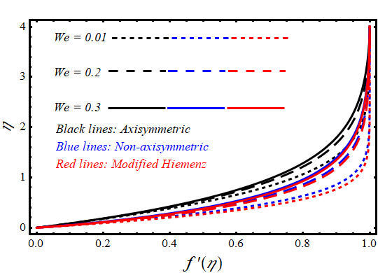
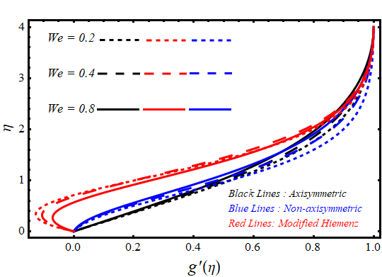
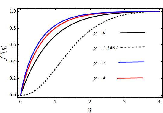
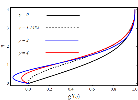
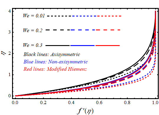
The behaviour is observed for $\gamma=0$ and $\gamma=2$ . It is clear that from Figure 1, at a particular point of $\eta$ , $f^{\prime}(\eta)$ , the velocity along x axis increases with the increase of $W e$ . Since $W e$ is the ratio of elastic forces to viscous forces, so because of their elasticity, viscoelastic fluids may store and release energy. The elastic effects grow more clear as the $W e$ number rises, allowing the fluid to store more energy. The fluid's velocity may increase as a result of the stored energy. Comparative analysis also describes that for the case of Axisymmetric stagnation point the velocity is rises faster as compared to the corresponding velocity profiles for the case of non-axisymmetric and modified Hiemenz stagnation point flow of second grade fluid. Figure 2 shows the variation in velocity profile $g^{\prime}(\eta)$ , with $\eta$ , for different values of Weissenberg number. It is clear from Figure 2, at a particular point of $\eta$ , $g^{\prime}(\eta)$ , the velocity along x axis increases with the increase of $W e$ . When $We=\{0.4,0.6,0.8\}$ then for the case of modified Hiemenz stagnation point flow, the velocity is greater as compared to the velocity profiles of non-axisymmetric stagnation point and axisymmetric stagnation point flow. Figure 3 shows the similarity profiles $f^{\prime}(\eta)$ for different positive values of $\gamma$ . The profile for $\gamma=0$ , is the axisymmetric stagnation point flow. The critical value for $\gamma_{c}=1.1482$ displayed as a dashed line in the velocity where $g^{\prime\prime}(0)=0.$ The velocity $f^{\prime}(\eta)$ along y axis is increases by increasing the large values of $\gamma$ . Also Figure 4 shows the similarity profiles for $g^{\prime}(\eta)$ for different positive values of $\gamma$ . The profile for which $g^{\prime\prime}(0)=0,$ for $\gamma_{c}=1.1482$ is plotted as dashed line. The velocity $g^{\prime}(\eta)$ along x axis is increases by increasing the large values of $\gamma$ .

5.2 Temperature Profile

Figure 5 Effect of Nb on

\theta(\eta)

other parameters are

Nt=0.3,Sc=1,\Pr=3

and

We=0.5

Figure 6 Effect of Nt on

\theta(\eta)

other parameters are

Nb=0.9,Sc=1,\Pr=3

and

We=0.5

Figure 7 Effect of Pr on

\theta(\eta)

other parameters are

Nt=0.1,Nb=0.5,Sc=0.1

and

We=0.6

Figure 8 Effect of Sc on

\theta(\eta)

other parameters are

Nt=0.5,Nb=0.9,\Pr=3

and

We=0.5

Figure 9 Effect of We on

\theta(\eta)

other parameters are

Nt=0.5,Nb=0.5,\Pr=2

and

Sc=0.1

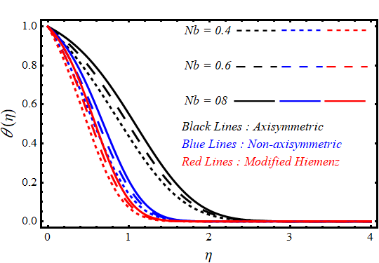
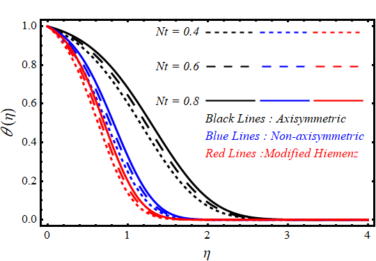
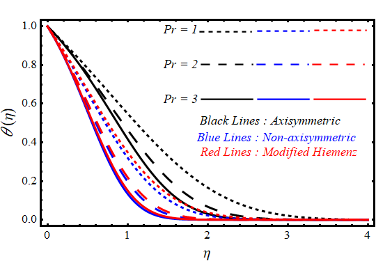
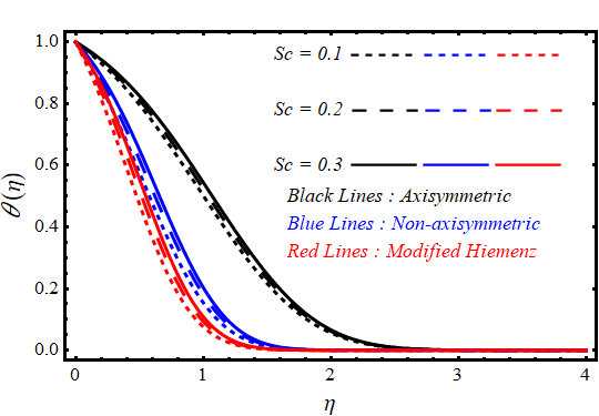
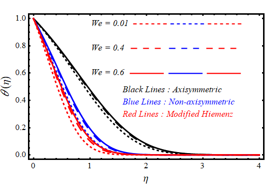
The effects of Weissenberg number $W e$ on the velocity distributions are presented in Figure 5 shows the influence of Brownian motion $N_{b}$ against $\theta(\eta)$ . Due to the fact that temperature is a measurement of the average kinetic energy of the molecules in a system, an increase in Brownian motion contributes to an increase in systemic temperature. The particles' kinetic energy is effectively increased as they move faster quickly and collide more energetically, transferring some of their energy to the suspended particles. The temperature rises as a result of the increased kinetic energy. So, higher the Brownian motion the quantity of temperature is rises. Comparative analysis also describes that for the case of Axisymmetric stagnation point the temperature is exceeded as compared to the corresponding temperature profiles for the case of non-axisymmetric and modified Hiemenz stagnation point flow of second grade fluid. Figure 6 shows the influence of Thermophoresis motion $N_{t}$ against $\theta(\eta)$ . It is clear from Figure 6, at a particular point of $\eta$ , $\theta(\eta)$ , the temperature along y axis increases with the increase of $N_{t}$ . When a fluid containing suspended particles is subjected to a temperature gradient, the particles feel a net force that pushes them from hot to cold areas of the fluid. The increase in temperature caused by the increase in thermophoresis is not a direct result of particle thermophoretic motion. Instead, it is the outcome of energy transfer that occurs during particle movement. Comparative analysis also illustrates that for the case of non-axisymmetric and modified Hiemenz stagnation point flow of second grade fluid the temperature profiles are smaller than the temperature of Axisymmetric stagnation point flow. Figure 7 shows the influence of Prandtl number $\Pr$ against $\theta(\eta)$ . Figure 7, at a particular point of $\eta$ , $\theta(\eta)$ , the temperature along y axis decreases with the increase of $\Pr$ . The thermal conductivity of the fluid decreases as the Prandtl number rises, and hence the temperature decreases. This is because a lower thermal diffusivity, indicated by a greater Prandtl number, means that heat transfer through the fluid occurs more slowly. Comparative analysis indicates that the temperature profile for axisymmetric stagnation point is smaller as compared to temperature profiles for non-axisymmetric stagnation point and modified stagnation point flow of second grade fluid by the increment in Prandtl number. The graphical relationship between the temperature profile $\theta(\eta)$ and the Schmidt number $S c$ is shown in Figure 8. It shows that at a particular point of $\eta$ , $\theta(\eta)$ , the temperature along y axis increases with the increase of $S c$ . Schmidt number is the ratio of viscous to molecular diffusion rate. When the Schmidt number is increased then a large viscous diffusion rate is observed. As a result, temperature profiles starts to grow. Comparative analysis indicates that the temperature profile for axisymmetric stagnation point is rises fast as compared to temperature profiles for non-axisymmetric stagnation point and modified stagnation point flow of second grade fluid by the increment of Schmidt number. Figure 9 shows the influence of Weissenberg number $W e$ against $\theta(\eta)$ . It shows that at a particular point of $\eta$ , $\theta(\eta)$ , the temperature along y axis increases with the increase of Weissenberg number $W e$ . Comparative analysis indicates that the temperature profile for axisymmetric stagnation point is rises fast as compared to temperature profiles for non-axisymmetric stagnation point and modified stagnation point flow of second grade fluid by the increment of Weissenberg number.

5.3 Concentration Profile

Figure 10 Effect of Nb on

\phi(\eta)

other parameters are

Nt=0.4,Sc=1,\Pr=3

and

We=0.5

Figure 11 Effect of Nt on

\phi(\eta)

other parameters are

Nb=0.9,Sc=0.1,\Pr=3

and

We=0.5

Figure 12 Effect of Pr on

\phi(\eta)

other parameters are

Nt=1,Sc=1,Nb=0.9

and

We=0.5

Figure 13 Effect of Sc on

\phi(\eta)

other parameters are

Nt=0.9,Nb=1,\Pr=4

and

We=0.2

Figure 14 Effect of

W e

\phi(\eta)

other parameters are

Nt=0.1,Nb=0.2,\Pr=3

and

Sc=3

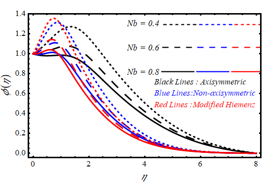
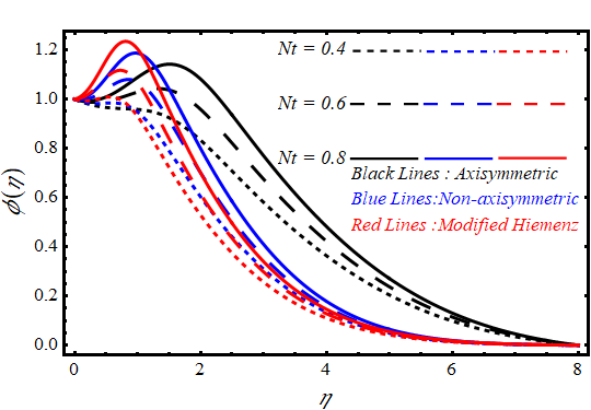
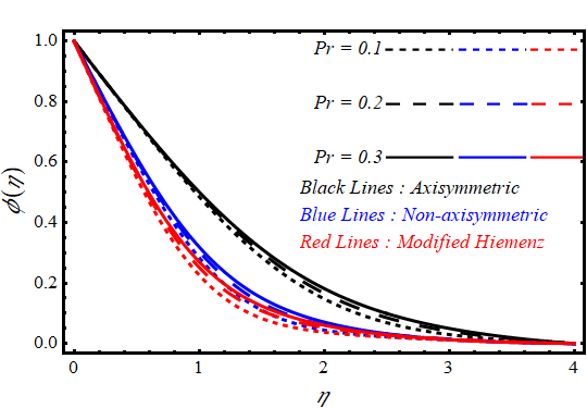
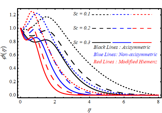
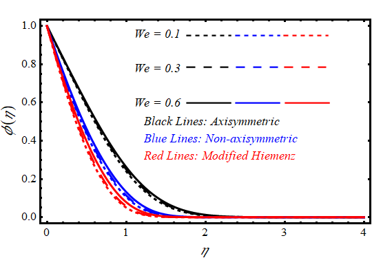
Figure 10 shows a graphical representation of the concentration profile $\phi(\eta)$ for various values of the $N b$ . Normally, the Brownian movement constraint Nb which arises due to the presence of nanoparticles. The concentration profile $\phi(\eta)$ gradually decreases as $N b$ increases for axisymmetric, non-axisymmetric and modified Hiemenz stagnation point flows. Actually, the nanoparticles are pushed by the Brownian effect in the direction of the concentration gradient. Lower the solutal field of nano fluid, larger the Brownian motion variable. Comparative analysis indicates that the temperature profile for modified Hiemenz stagnation point is greater as compared to concentration profiles for non-axisymmetric stagnation point and axisymmetric stagnation point flow of second grade fluid by the increment of Nb. Figure 11 shows a graphical representation of the concentration profile $\phi(\eta)$ for various values of $N t$ . For axisymmetric, non-axisymmetric and modified Hiemenz stagnation point, it can be shown that the concentration profile $\phi(\eta)$ rise with the higher amount of thermophoresis variable $N t$ . Physically, the thermophoresis phenomenon arises as a result of nanoparticles moving from hot region to cold region which causes the resulting nanoparticle's percentage to rise. Comparative analysis indicates that the concentration profile for modified Hiemenz stagnation point is greater as compared to concentration profiles for non-axisymmetric stagnation point and axisymmetric stagnation point flow of second grade fluid by the increment of Nb. Figure 12 captured the notable effect of $\Pr$ on the concentration profile $\phi(\eta)$ . As the value of dimensionless Prandtl number $\Pr$ increases the concentration profile $\phi(\eta)$ increases because the thermal boundary layer is closely related to the concentration profile. The concentration gradient across this layer is likewise steeper with larger Prandtl numbers because the thermal boundary layer is smaller. As a result, as the Prandtl number rises, the concentration profile grows more quickly. Through comparison, we notice that the amount of mass transfer is small in non-axisymmetric and modified stagnation point than the axisymmetric stagnation point.

The physical features of Schmidt number $S c$ and solutal field $\phi(\eta)$ are described in Figure 13. As the value of dimensionless $S c$ increases, the solutal field gradually starts decreasing for all three cases. Schmidt number is the ratio of viscous to molecular diffusion rate. When the Schmidt number is increased and the fluid concentration drops, a large viscous diffusion rate is observed. As a result, concentration profiles start to decline. Comparative analysis depicts that the concentration profile for modified Hiemenz stagnation point is greater as compared to concentration profiles for non-axisymmetric stagnation point and axisymmetric stagnation point flow of second grade. The physical features of Weissenberg number $W e$ and solutal field $\phi(\eta)$ are described in Figure 14. The concentration profile $\phi(\eta)$ is growing by increasing the values of Weissenberg number $W e$ . The distribution of solute or dispersed particles within the fluid is referred to as the concentration profile. The fluid is undergoing greater rates of shear and elastic deformation when the Weissenberg number rises. Although the behavior of viscoelastic fluids can be complicated, in general, a higher Weissenberg number results in more prominent elastic effects and flow-induced structure development. The concentration profile may be significantly impacted by these flow-induced structures.

5.4 Skin Friction

Figure 15 Influence of

W e

on velocity profile

f^{\prime\prime}(0)

and

g^{\prime\prime}(0)

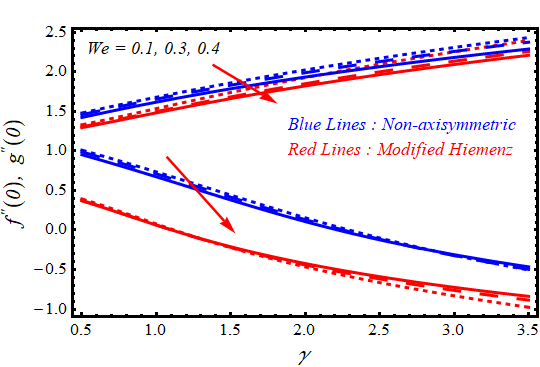
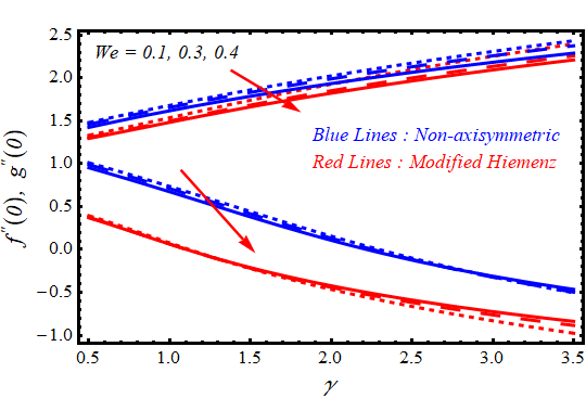
Figure 15 shows the behavior of Weissenberg number on the velocity profiles $f^{\prime\prime}(0)$ and $g^{\prime\prime}(0)$ . It is seen that an increase in $W e$ reduces the wall shear stress. The viscoelastic behavior of the fluid is enhanced by the stronger elastic effects as the Weissenberg number rises. When viscoelastic fluids deform, they have the capacity to store and release energy, altering the flow behavior. Longer relaxation times and a higher degree of elastic deformation are indicated by a rise in the Weissenberg number. Therefore, when the Weissenberg number rises, the flow is more affected by elastic processes, resulting in a fluid with lower effective viscosity and lower wall shear stress than in purely viscous flow. Comparative analysis indicates that the wall shear stress in non-axisymmetric stagnation point flow rapidly exceeds that of the modified stagnation point flow of second grade fluid (see Table 1).

Table 1 Comparison result for

f^{\prime\prime}(0)

and

[g^{\prime\prime}(0)]

for various values of

\gamma

and

W e

. Dashes (–) indicate that the value is not applicable or not computed.

$W e$	$\gamma$	Axisymmetric	Non-Axisymmetric	Modified Hiemenz
0.00001	0	1.31195	–	–
		[1.31195]	–	–
0.1		1.28304	–	–
		[1.28304]	–	–
0.5		1.2035	–	–
		[1.2035]	–	–
	1	–	1.6173261	1.4690242
		–	[0.67356834]	[0.06313222]
	2	–	1.9345877	1.7981013
		–	[0.10774733]	[-0.403979]
	3	–	2.1825311	2.0587613
		–	[-0.31044393]	[-0.686853]

Table 2 Comparison result of

\theta^{\prime}(0)

and

\phi^{\prime}(0)

for different values of

\Pr,\gamma,We,Sc,Nb

and

N t

. Dashes (–) indicate that the value is not applicable or not computed.

$W e$	$\gamma$	$\Pr$	$N b$	$N t$	$S c$	Axisymmetric	Non-axisymmetric	Modified Hiemenz
0.00001	0	1	0.9	0.5	0.5	0.432568	–	–
						[0.543449]	–	–
0.1						0.425155	–	–
						[0.534946]	–	–
0.5						0.405484	–	–
						[0.513243]	–	–
	1					–	0.481211	0.413012
						–	[0.635692]	[0.524302]
	2					–	0.547341	0.530011
						–	[0.699907]	[0.648106]
	3					–	0.634535	0.632623
						–	[0.79405]	[0.76957]
	2	1.5				–	0.545993	0.535725
						–	[0.725473]	[0.668277]
		2				–	0.524563	0.519602
						–	[0.760885]	[0.69958]
		3				–	0.460584	0.463058
						–	[0.839507]	[0.772374]
			0.6			–		0.509104
						–	[0.874389]	[0.50737]
			0.7			–	0.348233	0.456949
						–	[0.89506]	[0.552957]
			0.8			–	0.300837	0.408831
						–	[0.907107]	[0.584616]
				0.4		–	0.331977	0.443127
						–	[0.877014]	[0.573753]
				0.6		–	0.272871	0.377253
						–	[0.940416]	[0.600574]
				0.8		–	0.225219	0.3215
						–	[1.01349]	[0.644565]
					0.3	–	0.39501	0.412677
						–	[0.484123]	[0.401172]
					3	–	0.124736	0.124196
						–	[1.62777]	[1.57339]
					5	–	0.101964	0.10074
						–	[1.92883]	[1.87644]

5.5 Heat Transfer

Figure 16 Influence of

W e

on velocity profile

f^{\prime\prime}(0)

and

g^{\prime\prime}(0)

other parameters are

Nt=0.5,Nb=0.5,Sc=0.9

and

\Pr=3

Figure 17 Influence of

W e

on velocity profile

\theta^{\prime}(0)

other parameters are

Nt=0.5,Nb=0.5,Sc=0.9

and

\Pr=3

Figure 18 Influence of

N b

on velocity profile

\theta^{\prime}(0)

other parameters are

Nt=0.4,We=0.3,Sc=0.9

and

\Pr=3

Figure 19 Influence of

N t

on velocity profile

\theta^{\prime}(0)

other parameters are

We=0.3,Nb=0.8,Sc=0.9

and

\Pr=3

Figure 20 Influence of

\Pr

on velocity profile

\theta^{\prime}(0)

other parameters are

Nt=0.5,Nb=0.8,Sc=1

and

We=0.3

Figure 21 Influence of

S c

on velocity profile

\theta^{\prime}(0)

other parameters are

Nt=0.3,Nb=0.7,We=0.3

and

\Pr=3

5.6 Mass Transfer

Figure 22 Influence of

W e

on velocity profile

\phi^{\prime}(0)

when other parameters are

Nt=0.5,Nb=0.5,Sc=0.9

and

\Pr=3

Figure 23 Influence of

N b

on velocity profile

\phi^{\prime}(0)

when other parameters are

Nt=0.4,We=0.2,Sc=0.9

and

\Pr=0.4

Figure 24 Influence of

N t

on velocity profile

\phi^{\prime}(0)

when other parameters are

Nb=0.8,We=0.2,Sc=0.9

and

\Pr=0.4

Figure 25 Influence of

\Pr

on velocity profile

\phi^{\prime}(0)

when other parameters are

Nb=0.8,We=0.2,Sc=0.9

and

Nt=0.4

Figure 26 Influence of

S c

on velocity profile

\phi^{\prime}(0)

when other parameters are

Nt=0.4,We=0.2,\Pr=0.4

and

Nb=0.8

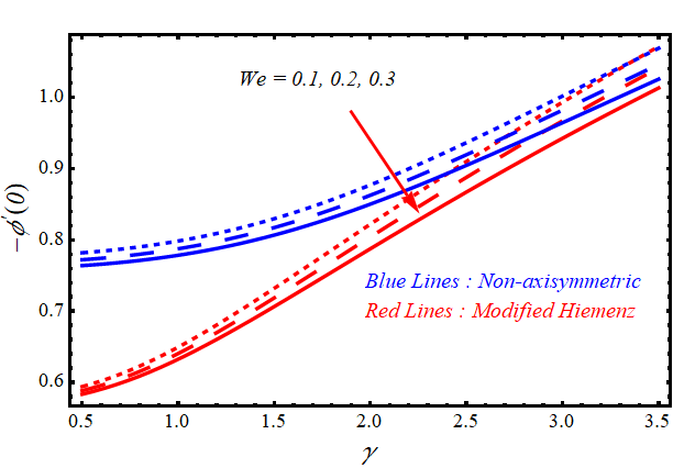
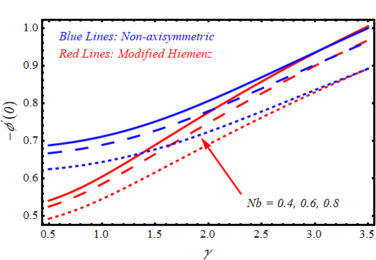
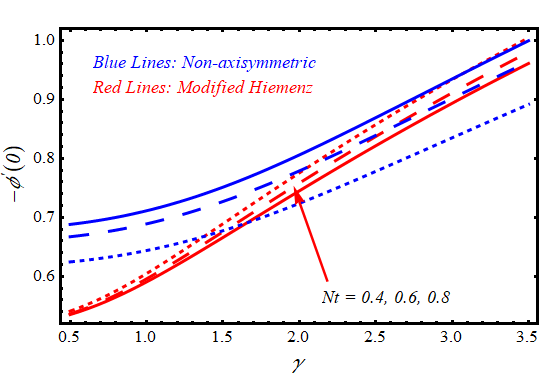
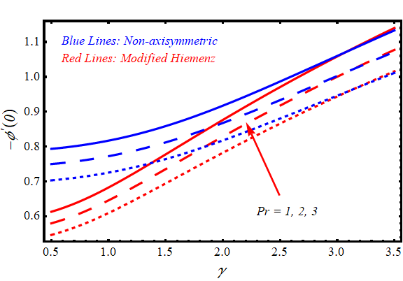
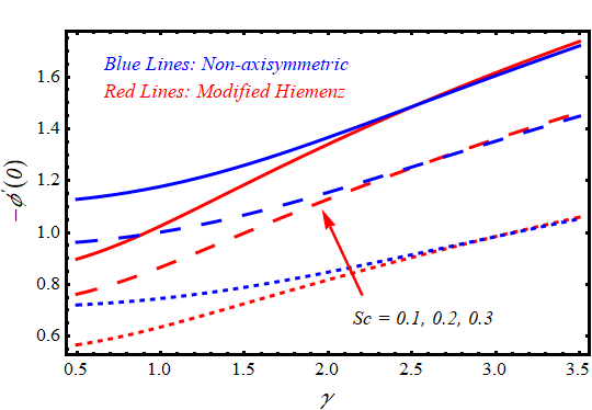
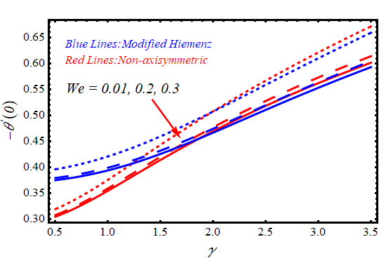
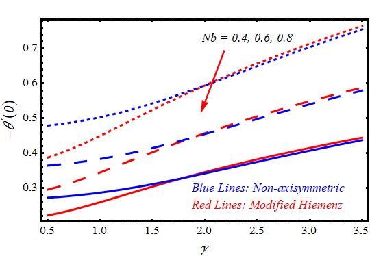
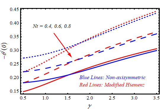
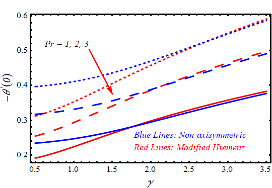
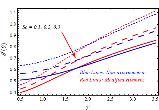
Figure 16 depicts the effect of dimensionless parameter $W e$ (Weissenberg number) on the local Nusselt number $Nu_{x}(Re_{x})^{-\frac{1}{2}}$ . Here local heat transfer rate is the decreasing function of $W e$ . This is due to a few factors. First, the fluid flow can be restricted by elastic forces, slowing the rate of heat transfer. Second, the fluid may develop a "skin" close to the heat transfer surface as a result of the elastic stresses, which can also slow down the rate of heat transmission. Third, the fluid may have a more complicated flow pattern as a result of the elastic forces, which could make it harder for heat to pass from the surface to the fluid. As a result of these considerations the local heat transfer rate will decrease as the Weissenberg number rises. The influence of Brownian motion $N_{b}$ on the local Nusselt number $Nu_{x}(Re_{x})^{-\frac{1}{2}}$ is displayed in Figure 17. It is clear that local heat transfer rate is decreasing function of Brownian motion $N b$ . The temperature gradient at the surface is decreased as a result of the increased Brownian motion, which leads the nanoparticles to diffuse away from the hot surface because of this the local heat transfer coefficient slows down as the Brownian motion parameter rises. Figure 18 depicts the the influence of Thermophoresis motion $N_{t}$ on the local Nusselt number $Nu_{x}(Re_{x})^{-\frac{1}{2}}$ . We can observed that local heat transfer rate is the decreasing function of parameter of Thermophoresis motion $N_{t}$ . Since, the inverse relationship exist between local heat transfer rate and thermophoresis motion. So, local heat transfer decreases by an increasing the thermophoresis motion parameter. The particles in the fluid are more likely to move the heated surface when thermophoresis motion increases. As a result, there will be a small number of particles available to transmit heat away from the surface, which will slow down the rate of heat transfer. Figure 19 displayed the effect of Prandtl number $\Pr$ on the local Nusselt number $Nu_{x}(Re_{x})^{-\frac{1}{2}}$ . It is clear that the wall heat transfer rate is the decreasing function of $\Pr$ . The rate at which heat is transferred from a surface to a fluid passing by it is known as the local heat transfer rate. It is a Prandtl number's function, and it gets smaller as the Prandtl number rises. This is because a higher Prandtl number indicates that the fluid is more viscous, which causes the heat to flow through the fluid to take longer. The local heat transmission rate is consequently reduced. The graphical relationship between the local Nusselt number $Nu_{x}(Re_{x})^{-\frac{1}{2}}$ and the Schmidt number $S c$ is shown in Figure 20. We can observed that the wall heat transfer is decays when Schmidt number increases. As the Schmidt number increases, the Nusselt number decreases so local heat transfer rate decays. A higher Schmidt number indicates that the fluid diffuses more slowly. As a result a lower local heat transfer rate is achieved since it will take longer for the heat to flow from the fluid's surface to its inside. Figure 21 illustrates the effect of the strain-to-shear ratio $\gamma$ on the local Nusselt number $Nu_{x}(Re_{x})^{-\frac{1}{2}}$ . It is observed that an increase in $\gamma$ leads to a reduction in the local heat transfer rate, as the altered flow dynamics induced by the strain-to-shear ratio affect the thermal boundary layer, thereby reducing the efficiency of heat transfer from the surface to the fluid.

From comparative analysis, we can conclude that by increasing the dimensionless parameters $\Pr,We,Sc,Nb$ and $N t$ the wall heat transfer rate is larger in non-axisymmetric stagnation point flow than the modified Hiemenz stagnation point flow of second grade fluid.

Figure 22 displays the effects of $W e$ on the local Sherwood number $Sh_{x}(Re_{x})^{-\frac{1}{2}}$ . We can see that local mass transfer rate is the decreasing function of Weissenberg number $W e$ . The elastic forces become more dominant by increasing the Weissenberg number, which may prevent the ability of the fluid to transfer mass. This is because the fluid may become more structured as a result of the elastic forces, which makes it more challenging for the fluid molecules to move around and interact with one another. As a result, the Weissenberg number rises, the local mass transfer rate will decrease. Figure 23 displays the effects of parameter of Brownian motion $N_{b}$ on the local Sherwood number $Sh_{x}(Re_{x})^{-\frac{1}{2}}$ . Here local mass transfer rate is increasing function of $N_{b}$ . A larger local mass transfer rate will result from stronger Brownian motion, which is indicated by a higher value of $N b$ . Because of this the stronger Brownian motion will cause the nanoparticles to move more quickly between phases. The nanoparticles move erratically (random) due to Brownian motion. More collisions and more mass transfer will take place when Brownian motion becomes stronger. Because of this, Brownian motion $N b$ and the local mass transfer rate are both rising functions.

Figure 24 shows the effects of parameter of Thermophoresis motion $N_{t}$ on the local Sherwood number $Sh_{x}(Re_{x})^{-\frac{1}{2}}$ . It is clear that rate of transfer of mass is the increasing function of Brownian motion $N_{b}$ . There is an increase in the local mass transfer rate by increasing the thermophoresis motion because as $N t$ increases, thermophoresis becomes faster, which leads to to an increase in the migration of nanoparticles to the surface and a steeper concentration gradient near the surface. This both contribute to an increase in the local mass transfer rate. The graphical relationship between the local Sherwood number $Sh_{x}(Re_{x})^{-\frac{1}{2}}$ and the Prandtl number $\Pr$ is shown in Figure 25. We can see that the rate of transfer of mass is an increasing function of Prandtl number $\Pr$ . There is a direct relationship between local Sherwood number $Sh_{x}(Re_{x})^{-\frac{1}{2}}$ and the Prandtl number $\Pr$ . A larger Prandtl number means that the diffusivity of momentum is low. This means that the fluid will have a harder time resisting the forces that are driving the mass transfer, so the rate of mass transfer will also rise. The influence of Schmidt number $S c$ on the local Sherwood number $Sh_{x}(Re_{x})^{-\frac{1}{2}}$ is displayed in Figure 26. We can observed that the rate of transfer of mass is an increasing function of Schmidt number $S c$ . A greater Schmidt number causes steeper concentration gradients close to the interface, which in turn promotes quicker mass transfer across the boundary or interface. As a result, the wall mass transfer rate is an increasing function of the Schmidt number.

From comparative analysis, we can conclude that by increasing the dimensionless parameters $\Pr$ , $S c$ , $N b$ , and $N t$ , the wall mass transfer rate is larger in non-axisymmetric stagnation point flow than the modified Hiemenz stagnation point flow of second grade fluid, while the mass transfer rate decreases with increasing $W e$ . The numerical results presented in Table 2, validate the effects of these parameters on the local Sherwood number.

6. Main Findings

The velocity $f^{\prime}(\eta)$ , concentration and temperature profiles increases by an increasing the values of $W e$ .
The velocity $g^{\prime}(\eta)$ decreases by an increasing the values of $W e$ .
By increasing Brownian parameter $N_{b}$ , the temperature is increased while opposite behavior is achieved for concentration.
By increasing thermophoresis parameter $N_{t}$ , both concentration and temperature profiles rises.
For large values of Prandtl number $\Pr$ , the temperature is declined while opposite behavior is achieved in concentration.
The temperature is exceeds for increasing values of Schmidt number $S c$ , while concentration profile is declined.
The wall shear stresses $f^{\prime\prime}(0)$ and $g^{\prime\prime}(0)$ are decreasing function of $W e$ .
The local heat transfer rate is an decreasing function of $N b, N t, W e, S C$ and $\Pr$ .
The local mass transfer rate is an increasing function of $N b, N t, S C$ and $\Pr$ while opposite trend is obtained for $W e$ .

Data Availability Statement

Data will be made available on request.

Funding

This work was supported without any funding.

Conflicts of Interest

The authors declare no conflicts of interest.

Ethical Approval and Consent to Participate

Not applicable.

References

Hiemenz, K. (1911). Die Grenzschicht an einem in den gleichformigen Flussigkeitsstrom eingetauchten geraden kreiszylinder. Gottingen dissertation. Dingler's polytech. J, 326, 311.
Google Scholar
Ariel, P. D. (1995). A numerical algorithm for computing the stagnation point flow of a second grade fluid with/without suction. Journal of Computational and Applied Mathematics, 59(1), 9-24.
CrossRef Google Scholar
Ariel, P. D. (2001). Axisymmetric flow of a second grade fluid past a stretching sheet. International Journal of Engineering Science, 39(5), 529-553.
CrossRef Google Scholar
Ariel, P. D. (2002). On extra boundary condition in the stagnation point flow of a second grade fluid. International Journal of Engineering Science, 40(2), 145-162.
CrossRef Google Scholar
Attia, H. A. (2003). Homann magnetic flow and heat transfer with uniform suction or injection. Canadian Journal of Physics, 81(10), 1223-1230.
CrossRef Google Scholar
Barış, S., & Dokuz, M. S. (2006). Three-dimensional stagnation point flow of a second grade fluid towards a moving plate. International Journal of Engineering Science, 44(1-2), 49-58.
CrossRef Google Scholar
Dunn, J. E., & Fosdick, R. L. (1974). Thermodynamics, stability, and boundedness of fluids of complexity 2 and fluids of second grade. Archive for Rational mechanics and Analysis, 56(3), 191-252.
CrossRef Google Scholar
Gorla, R. S. R. (1978). Nonsimilar axisymmetric stagnation flow on a moving cylinder. International Journal of Engineering Science, 16(6), 397-400.
CrossRef Google Scholar
Hayat, T., Anwar, M. S., Farooq, M., & Alsaedi, A. (2014). MHD stagnation point flow of second grade fluid over a stretching cylinder with heat and mass transfer. International Journal of Nonlinear Sciences and Numerical Simulation, 15(6), 365-376.
CrossRef Google Scholar
Ahmad, M., Ahmad, I., & Sajid, M. (2016). Heat transfer analysis in an axisymmetric stagnation-point flow of second grade fluid over a lubricated surface. American Journal of Heat and Mass Transfer, 3(1), 1-14.
Google Scholar
Homann, F. (1936). Einfluß großer zähigkeit bei strömung um zylinder. Forschung auf dem Gebiet des Ingenieurwesens A, 7(1), 1-10.
CrossRef Google Scholar
Ishihara, Y., & Paullet, J. E. (2008). Dual solutions for axisymmetric stagnation point flow over a lubricated surface. Communications in Applied Analysis, 12(3), 289-296.
Google Scholar
Khan, M., El Shafey, A. M., Salahuddin, T., & Khan, F. (2020). Chemically Homann stagnation point flow of Carreau fluid. Physica A: Statistical Mechanics and its Applications, 551, 124066.
CrossRef Google Scholar
Khan, M., Sarfraz, M., Ahmed, J., Ahmad, L., & Fetecau, C. (2020). Non-axisymmetric Homann stagnation-point flow of Walter’s B nanofluid over a cylindrical disk. Applied Mathematics and Mechanics, 41(5), 725-740.
CrossRef Google Scholar
Labropulu, F., & Li, D. (2008). Stagnation-point flow of a second-grade fluid with slip. International Journal of Non-Linear Mechanics, 43(9), 941-947.
CrossRef Google Scholar
Libby, P. A. (1962). The homogeneous boundary layer at an axisymmetric stagnation point with large rates of injection. Journal of the Aerospace Sciences, 29(1), 48-60.
CrossRef Google Scholar
Lin, T. C., & Schaaf, S. A. (1951). Effect of slip on flow near a stagnation point and in a boundary layer (No. NACA-TN-2568).
Google Scholar
Mahabaleshwar, U. S., Nagaraju, K. R., Nadagoud, M. N., Bennacer, R., & Baleanu, D. (2020). An MHD viscous liquid stagnation point flow and heat transfer with thermal radiation and transpiration. Thermal Science and Engineering Progress, 16, 100379.
CrossRef Google Scholar
Nadeem, S., Ishtiaq, B., Almutairi, S., & Ghazwani, H. A. (2022). Impact of Cattaneo–Christov double diffusion on 3d stagnation point axisymmetric flow of second-grade nanofluid towards a riga plate. International Journal of Modern Physics B, 36(29), 2250205.
CrossRef Google Scholar
Nawaz, M., Alsaedi, A., Hayat, T., & Alhothauli, M. S. (2013). Dufour and Soret effects in an axisymmetric stagnation point flow of second grade fluid with newtonian heating. Journal of Mechanics, 29(1), 27-34.
CrossRef Google Scholar
Rahimi, A. B., & Saleh, R. (2007). Axisymmetric Stagnation—Point Flow and Heat Transfer of a Viscous Fluid on a Rotating Cylinder With Time-Dependent Angular Velocity and Uniform Transpiration. Journal of Fluids Engineering, 129(1), 106-115.
CrossRef Google Scholar
Rott, N. (1956). Unsteady viscous flow in the vicinity of a stagnation point. Quarterly of Applied Mathematics, 13(4), 444-451.
Google Scholar
Sahoo, B., & Labropulu, F. (2012). Steady Homann flow and heat transfer of an electrically conducting second grade fluid. Computers & Mathematics with Applications, 63(7), 1244-1255.
CrossRef Google Scholar
Saif, R. S., Hayat, T., Ellahi, R., Muhammad, T., & Alsaedi, A. (2017). Stagnation-point flow of second grade nanofluid towards a nonlinear stretching surface with variable thickness. Results in physics, 7, 2821-2830.
CrossRef Google Scholar
Sajid, M., Mahmood, K., & Abbas, Z. (2012). Axisymmetric stagnation-point flow with a general slip boundary condition over a lubricated surface. Chinese Physics Letters, 29(2), 024702.
CrossRef Google Scholar
Saleh, R., & Rahimi, A. B. (2004). Axisymmetric stagnation-point flow and heat transfer of a viscous fluid on a moving cylinder with time-dependent axial velocity and uniform transpiration. Journal of Fluids Engineering, 126(6), 997-1005.
CrossRef Google Scholar
Santra, B., Dandapat, B. S., & Andersson, H. I. (2007). Axisymmetric stagnation-point flow over a lubricated surface. Acta Mechanica, 194(1), 1-10.
CrossRef Google Scholar
Takhar, H. S., Chamkha, A. J., & Nath, G. (1999). Unsteady axisymmetric stagnation-point flow of a viscous fluid on a cylinder. International Journal of Engineering Science, 37(15), 1943-1957.
CrossRef Google Scholar
Wang, C. Y. (1973). Axisymmetric stagnation flow towards a moving plate. AIChE Journal, 19(5), 1080-1081.
CrossRef Google Scholar
Weidman, P. (2014). Axisymmetric stagnation-point flow on a spiraling disk. Physics of Fluids, 26(7).
CrossRef Google Scholar
Weidman, P. D., & Mahalingam, S. (1997). Axisymmetric stagnation-point flow impinging on a transversely oscillating plate with suction. Journal of Engineering Mathematics, 31(2), 305-318.
CrossRef Google Scholar
Weidman, P. D. (2021). Three‐dimensional Hiemenz stagnation‐point flows. ZAMM‐Journal of Applied Mathematics and Mechanics/Zeitschrift für Angewandte Mathematik und Mechanik, 101(2), e201900319.
CrossRef Google Scholar
Zhong, Y., & Fang, T. (2011). Unsteady stagnation-point flow over a plate moving along the direction of flow impingement. International journal of heat and mass transfer, 54(15-16), 3103-3108.
CrossRef Google Scholar
Ziabakhsh, Z., Domairry, G., & Ghazizadeh, H. R. (2009). Analytical solution of the stagnation-point flow in a porous medium by using the homotopy analysis method. Journal of the Taiwan Institute of Chemical Engineers, 40(1), 91-97.
CrossRef Google Scholar

Cite This Article

APA Style

Abbasi, A. K., Ali, A. B. M., Naseer, M., Farooq, W., Ali, S., & Rafiq, M. (2025). Modified Hiemenz Stagnation Point Flow of Second Grade Nano Fluid. ICCK Journal of Applied Mathematics, 1(2), 66–85. https://doi.org/10.62762/JAM.2025.411313

Export Citation

RIS Format

Compatible with EndNote, Zotero, Mendeley, and other reference managers

BibTeX Format

Compatible with LaTeX, BibTeX, and other reference managers

Article Metrics

Citations:

Google Scholar

Crossref

Scopus

Web of Science

Article Access Statistics:

PDF Downloads: 1642

Publisher's Note

ICCK stays neutral with regard to jurisdictional claims in published maps and institutional affiliations.

Rights and Permissions

This article is an open access article distributed under the terms and conditions of the Creative Commons Attribution (CC BY) license.

Modified Hiemenz Stagnation Point Flow of Second Grade Nano Fluid

Abstract

Graphical Abstract

Keywords

1. Introduction

2. Flow Model

3. Physical Quantities of Interests

3.1 Similarity Transformations

4. Solution by Keller Box Method

4.1 Discritization Using Central Difference Approximation

5. Graphical Discussion and Results

5.1 Velocity

5.2 Temperature Profile

5.3 Concentration Profile

5.4 Skin Friction

5.5 Heat Transfer

5.6 Mass Transfer

6. Main Findings

Data Availability Statement

Funding

Conflicts of Interest

Ethical Approval and Consent to Participate

References

Cite This Article

Article Metrics

Google Scholar

Crossref

Scopus

Web of Science

Publisher's Note

Rights and Permissions

Table of Content

Current Issue

Volume 1, Issue 2

Journal Info

ICCK Journal of Applied Mathematics

XML Format

JATS XML

Article QR Code

Submit Your Research

Popular Articles