GPS Tracking Based on Stacked-Serial LSTM Network

Xuebo Jin; Songzheng Liu; Jianlei Kong; Yuting Bai; Tingli Su; Huijun Ma

doi:10.62762/CJIF.2024.361889

Abstract

Maneuvering target tracking, as a core task in multi-sensor information fusion, is widely used in unmanned vehicles, missile navigation, and underwater ship localization, where real-time and robust state estimation is critical. Due to the uncertainty of the moving characteristics of maneuvering targets and the low sensor measurement accuracy, trajectory tracking has always been an open research problem and challenging work. This paper proposes a Bayesian-inspired stacked LSTM fusion network (SLSTM) for uncertain motion characteristics. The network consists of two LSTM fusion networks with stacked serial relationships, one of which is used to predict the movement dynamics, and the other is used to update the track's state. Compared with the classical Kalman filter based on the maneuver model, the method proposed here does not need to model the motion characteristics and sensor characteristics. It can achieve high-performance tracking by learning historical data dynamics and sensor characteristics. Experimental results show that this method can effectively improve the trajectory estimation performance when the target motion is unknown and uncertain.

Graphical Abstract

GPS Tracking Based on Stacked-Serial LSTM Network

Click image to view fullscreen

Keywords

trajectory estimation recurrent neural network GPS filtering algorithm LSTM fusion networks stacked serial structure

1. Introduction

Global Positioning System (GPS) is a satellite navigation system that provides real-time position and speed information for moving targets [1]. However, GPS signals are imperfected and often affected by various external factors such as atmospheric conditions, satellite configuration, and receiver quality, resulting in noise in the measurements. This noise is not entirely random and can exhibit colored characteristics, with pink noise being one of the most prevalent types of noise in GPS signals. Pink noise has a higher power density at lower frequencies and gradually decreases as frequency increases. Its presence in GPS measurements can significantly affect the accuracy and precision of GPS-based tracking systems. As a classical method for GPS tracking, the Kalman filter is a linear minimum variance estimation under the discrete state space model with the system's dynamic and measurement equation. Classical filtering methods include the Kalman filter (KF), extended Kalman filter (EKF) [2], unscented Kalman filter (UKF) [3, 4, 5], volumetric Kalman filter (CKF) [6, 7], particle filter (PF) [8], etc. The accurate system models are particularly critical for tracking the performance of the Kalman series filters. In order to achieve precise tracking, it is necessary to establish a motion model that matches the actual state of the target motion. Current motion models mainly to include single-model and multiple-model methods. The single models have Constant Velocity (CV) [9], Constant Acceleration (CA) [10], Singer model [11], and Current Statistical (CS) model [12]. The CV and CA models consider the acceleration and derivative of maneuvering targets as zero-mean Gaussian noise, respectively, which fails to capture the targets' maneuvering behavior accurately. Singer model can give the acceleration of the maneuvering target as exponential autocorrelation zero mean colored noise, and its assumption of zero means is unreasonable for describing the moving state of the maneuvering target of actual situations. CS model improves the adaptive non-zero mean acceleration based on the Singer model and describes the statistical distribution characteristics of maneuvering acceleration according to the change of its mean value. However, the unreasonable setting will increase target tracking error because it needs to set the maneuvering frequency and acceleration limited in advance.

The single model method only uses one model to represent the system's motion mode, so it only applies to the system with a single motion mode and weak mobility. With the rapid improvement of the maneuverability of the target, the complex movement of the target makes it difficult for a single model to describe accurately, so the multi-model algorithm has been applied in many fields. The multi-model method uses multiple models to cover the numerous different motion modes of the target. Each model matches a motion model, and the outputs of all models are combined into the final state estimation of the target according to different weights. The interactive Multiple Model (IMM) [13] and adaptive interactive multiple models (AIMM) [14] are classic methods of multiple model algorithms. However, the multi-model algorithm contains more models, reducing the performance and increasing the computational load.

The classical Kalman filtering algorithm enhances tracking accuracy by incorporating motion characteristics and dynamics into its model and using observations to correct estimation results. However, accurate modeling can be challenging due to the complexities of maneuvering target motion. As a result, over-reliance on the model has become a significant weakness of the algorithm.

The development of deep neural networks in recent years has led to significant advancements in tracking applications. Deep neural networks can learn discriminant features from big data, unlike traditional model-based methods. Data uncertainty and noise can be effectively dealt with by choosing an appropriate neural network. The recurrent neural network (RNN) is a widely used time series data network. However, RNN's simple structure can result in gradient disappearance or explosion as the time horizon increases.

In contrast to RNN, Long short-term memory (LSTM) [15] networks have more forgotten gates that effectively address the problems of RNN's gradient disappearance and explosion and have a long-term memory function. LSTM performs better in extracting practical information from time series data and has high precision in estimating trajectories from measured values. For instance, Chen et al. [16] proposed IONet,which predicts the indoor trajectory of pedestrians by simultaneously processing IMU and GPS data using a multi-layer convolutional neural network (CNN) and an LSTM. The CNN extracts discriminant visual features from the mobile device's accelerometer and gyroscope signals, and the LSTM performs spatiotemporal modeling. Finally, IONet outputs the polar coordinate of pedestrians. Another example is AtLoc proposed by Wang et al. [17], which uses an attention mechanism to focus the network on the objects' features, improving the performance of motion target attitude regression. Utilizing deep neural networks enables the models to have better tracking accuracy. It reduces the reliance on handcrafted models, which can be limited by the availability of data and knowledge of the target motion behavior.

In recent years, there has been significant progress in predicting the GPS position information of moving targets using neural networks [18, 19, 20]. While these models have demonstrated good accuracy and robustness, their prediction process is akin to a "black box" and lacks interpretability, unlike the Kalman filter, which operates based on a model and provides an interpretable process for prediction and recursive optimization.

This paper presents the following main innovations:

(1) Incorporating the variational method into the classical LSTM weights training method in the proposed network offers a significant advantage by allowing the network to adapt to the colored pink noise of GPS signals. The method's ability to model uncertainty and adjust the network's weights accordingly helps overcome the detrimental effects of such noise on the accuracy of GPS-based tracking systems. By improving the capability of LSTM to fuse the colored nature of GPS signal noise, the proposed method enhances tracking performance. It provides a more robust solution for GPS-based tracking applications.

(2) The proposed stacked LSTM structure is designed to estimate tracking trajectories while avoiding the need for modeling moving objects, which sets it apart from the Kalman filter. Unlike traditional neural networks, the prediction process of the proposed method involves a unique prediction and upload step, which offers improved interpretability. This design also takes advantage of the LSTM's long-term memory to capture the sequence dependencies of GPS measurements, leading to superior estimation performance compared to the Kalman filter.

2. Related Work

Kalman filter and its variants have been widely applied in moving target tracking. They are one of the most commonly used filtering methods due to their advantages in the real-time estimation of statistical parameters of the system and observation of noise through searching the minimum mean squared error. Specifically, for estimating the motion position and velocity of moving targets based on GPS, the Kalman filter can utilize the positional information obtained from GPS as the state observation and fuse it with the kinematic model to achieve more accurate estimation results. Moreover, improved Kalman filters, such as the extended Kalman filter, can handle non-linear systems dynamic models, which makes them more suitable for complex motion trajectories. Although Kalman filter has limitations in dealing with certain problems, such as multiple types of noise and insufficient prior information, incorporating other estimation algorithms and deep learning techniques can further extend its functionality and application. For example, Sun et al. [21] proposed an adaptive Kalman filter that combines the volumetric Kalman filter with the Sage Husa estimator for moving target tracking. This new algorithm enables real-time estimation of the statistical parameters and observation noise of unknown systems, thus avoiding algorithm divergence.

Additionally, it can reduce tracking error caused by unusual noise while improving accuracy and numerical stability. By introducing the Sage Husa estimator into the volume Kalman filter algorithm, the proposed adaptive Kalman filter offers a superior approach for moving target tracking. Nagui et al. [22] designed a cascaded extended Kalman filter to couple GPS and INS. The original GPS data is fused with the noisy Euler angle from the inertial measurement unit to produce more consistent and accurate real-time position information. Sun et al. [23] proposed a Marginal Kalman Filter (MKF) algorithm for maneuvering target tracking that models the system's nonlinear measurement equation as a weighted sum of Hermite polynomials. The algorithm estimates the prior distribution of the weighting matrix as a Gauss process. It calculates its posterior distribution, which is then used to remove the influence of the weighting matrix by calculating its integral. In order to improve the stability of the MKF algorithm, a strong tracking filter is introduced by using fading factors in the MKF algorithm, which can reduce the impact of previous filtering steps on the current step. Huang et al. [24] proposed a new adaptive Kalman filter based on the variable Bayesian theory. By selecting the inverse Wishart prior matrix and inferring the covariance matrix of state, prediction error, and measurement noise based on the variable Bayesian method, the structure has better robustness and can resist the process and measurement noise covariance. Chang et al. [25] designed a new fuzzy strong tracking cubature Kalman filter (FSTCKF) data fusion algorithm for the strong tracking Kalman Filter design. This algorithm enhances the filter's ability to identify and respond to dynamics. This algorithm can improve the positioning accuracy and stability of INS/GNSS integrated navigation system.

Although the previous research utilizing filtering methods can enhance the filtering capability of Kalman filter towards nonlinear and non-Gaussian White noise to a certain extent, its application may lead to filter divergence due to the target's sudden maneuvering motion, which may cause model mismatching issues.

In recent years, with the continuous development of deep learning, some researchers have combined deep learning to propose new target-tracking methods. Deep learning methods are widely used modeling methods, including RNNs, encoder-decoder, and other structures. This method combines massive training data and the computer's large-scale computing ability to optimize the model's internal parameters. It can fit complex nonlinear data, widely used in many fields [26, 27, 28]. Liu et al. [29] proposed the DeepMTT network with bidirectional LSTM using self-built mass offline trajectory data to pre-train the model. Zhang et al. [30] designed a trajectory-tracking model combining LSTM with the Unscented Kalman Filter (UKF). They used the autonomous learning and memory characteristics of the LSTM network to provide the UKF algorithm with predictive observation values. The simulation results show that the LSTM UKF algorithm model has a good tracking effect. Li et al. [31] proposed a trajectory recognition method based on LSTM and a maneuver tracking method matching CS model parameters. This method uses LSTM to effectively combine the above information's characteristics to recognize the target motion state. The optimal filtering parameters of each motion mode are obtained through clustering analysis, and filtering is performed according to the identification results of the LSTM. Compared with the traditional maneuvering tracking model, this method can maintain a stable filtering gain during the maneuvering process. Yaqi et al. [32] designed a new filter with a feedforward neural network, RNN, and attention mechanism. Vedula et al. [33] compared the classical tracking technology and LSTM deep learning model in the maneuvering target tracking application. Giuliari et al. [34] established a motion trajectory tracking model based on the transformer model, combining the codec and attention mechanism, and the model verifies the performance on multiple trajectory prediction benchmarks such as TrajNet [35]. James [36] proposed a tracking mode recognition mechanism based on the development of discrete wavelet transform and deep learning. Discrete wavelet transform offers time-frequency characteristics and assists neural network classification and prediction. Liu [37] proposed a Gaussian mixture model and Kullback Leibler's deep learning framework with multiple LSTMs to predict the vehicle position and combined improved extended Kalman filter (IEKF) and multiple LSTMs to optimize the vehicle positioning accuracy. The application of these models improves the tracking performance and proves the feasibility and effectiveness of using deep learning data-driven methods for target tracking. The traditional weak signal acquisition method cannot work correctly and accurately under various conditions. Moradi et al. [38] proposed a method based on deep convolutional neural networks and post collection to solve the problem of Doppler and navigation bit symbol conversion and in environments that do not meet nominal conditions. Taghizadeh et al. [39] proposed an architecture consisting of a set of layered LSTM and attention mechanisms to achieve long-term multi-stage prediction. In the absence of a GNSS network, this method can provide long-term navigation for drones and estimate their future state. He et al. [40] used the LSTM model to predict the Beidou satellite SCB, which improved the prediction accuracy of the Beidou-3 SCB. It reduces the impact of positioning errors and improves the accuracy of orbit determination. Orouji [41] proposed a multilayer perceptron neural network to track the trend of data, aiming at the fact that the estimator will lose tracking of the real signal when it does not know the characteristics of the GPS signal, and improve the accuracy of the GPS received signal by estimating the real trend. The above methods directly use the deep neural network for learning, take the measured data and the reference state to be estimated as the input and output networks, respectively, and directly obtain the desired state output through network training.

This paper proposes a novel stacked LSTM network for GPS position estimation that utilizes a deep learning method based on Bayesian variational inference. The proposed method incorporates the variational method into the classical LSTM weight training method to facilitate the adjustment of the network's weights according to the colored pink noise of GPS signals. By exploiting the LSTM's long-term memory to capture sequence dependencies, the proposed method avoids the need to model moving objects, providing improved interpretability. Moreover, the ability of the proposed method to handle colored GPS signal noise improves tracking performance and provides a robust solution for GPS-based tracking applications. Overall, the proposed method effectively extracts dynamic motion characteristics to model colored noise, enhancing the accuracy and performance of deep learning models for complex maneuvering scenarios.

3. Stacked LSTM Fusion Tracking Model

3.1 Bayesian Estimation

The essence of trajectory estimation is to estimate the state of the moving target according to the sensor's measurement. In the traditional model-based estimation method, it is assumed that the moving target and the corresponding measured value have a known mathematical model representation with sufficient accuracy, which is usually expressed by the following Equation (1):

{X_{t+1}}=f\left({{X_{t}}}\right)+{w_{\rm{t}}}

where $X_{t}$ is the state vector of the first time step of the moving target, is the process noise, and is the state transition function of the hypothetical model. It is assumed that the measured values depend on the model and are related to reality by the following Equation (2):

{Z_{t}}={h_{t}}\left({{X_{t}}}\right)+{q_{t}}

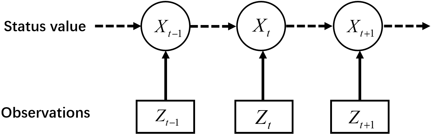
where $w_{t}$ is the measured value of the sensor, $h_{t}$ is the measurement function determined by the sensor, and $q_{t}$ is the measurement noise of the sensor. In the target movement process, the target's position is estimated by using the trajectory of the actual moving target (state equation) and the actual information observed by the sensor (observation equation). In practice, noise is unavoidable in both state and observation. Only the state equation or observation equation is used to estimate the trajectory of moving targets. As time passes, the error between the estimated trajectory and the actual trajectory of moving targets will become larger and larger. Bayesian filtering can reduce the uncertainty of trajectory estimation of moving targets. Bayesian filtering estimates the probability of a hidden state by observations with noise, that is a posteriori probability distribution. The moving process of the moving target can be seen as a random process. The Bayesian filtering network is shown in Figure 1.

Figure 1 Graphical representation of a Bayesian filtering process.

Assume $Z_{t}=(Z_{1},Z_{2},...Z_{t})$ is the measurement sequence. The goal of trajectory estimation is to determine the calculation $p(X_{t}|Z_{t-1})$ and $p(X_{t}|Z_{t})$ , corresponding to the prediction process and filtering process respectively, the prediction Equation (3) in Bayesian filtering is:

p\left({{X_{t}}|{Z_{1:t-1}}}\right)=\int p({X_{t}}|{Z_{t-1}})p({X_{t-1}}|{X_{1% :t-1}})d{X_{t-1}}

The prediction results reflect the posterior of the state before the time measurement. The filtering uses the posterior probability calculation obtained from the prediction. The filtering Equation (4) is:

p\left({{X_{t}}|{Z_{1:t-1}}}\right)=\eta p({Z_{t}}|{X_{t}})p({X_{t}}|{Z_{1:t-1% }})\

where $\eta$ is the normalized variable. The uncertainty of moving objects challenges trajectory estimation because accurate dynamic models cannot be obtained.

3.2 Kalman Filter

The essence of Bayesian estimation is to use the known information to predict the state's prior probability density with the system's prediction model, and then modify the latest observation data to obtain the posterior probability density. Kalman filter is an algorithm based on the idea of a Bayesian filter.

Kalman filter is an optimal autoregressive data processing algorithm. For many problems, the Kalman filter can obtain optimal estimation results. Assume that the process and measurement model of the discrete linear system is Equation (5):

\displaystyle{X_{t+1}}=A{X_{t}}+w(t)

\displaystyle{Z_{t}}=C{X_{t}}+v(t)

where $X_{t}$ is the quantity to be estimated, and $Z_{t}$ is the measurement data obtained through the sensor. Equation (7) is the process model of the system, which refers to the model that the state to be estimated in the system. $A$ is the process matrix. The state at the previous time is $X_{t}$ . The state at the next time, that is $t+1$ , will become $X_{t+1}$ . $w(t)$ is the process noise, which represents the degree of uncertainty in the process from $X_{t}$ to $X_{t+1}$ . is called the measurement model, $C$ is the measurement matrix, and $v(t)$ is the measurement noise. The Kalman filtering process is as follows (6) - (10):

{\hat{X}_{t|t-1}}=A{\hat{X}_{t-1|t-1}}\

{\hat{X}_{t|t}}={\hat{X}_{t|t-1}}+K[{Z_{t}}-C{\hat{X}_{t|t-1}}]\

K\left(t\right)={P_{t|t-1}}{C^{T}}{\left[{{C^{T}}{P_{t|t-1}}C+R}\right]^{-1}}\

{P_{t|t-1}}=A{P_{t-1|t-1}}{A^{T}}+Q\

{P_{t|t}}=[I-KC]{P_{t|t-1}}\

Equation (6) is the prediction equation, Equation (7) is the updating equation, and Equation (8) is the filtering gain equation and $K$ is the Kalman gain parameter; Equation (9) is the prediction equation of the next step, and $P_{t|t-1}$ is the estimated variance of $X_{t|t-1}$ ; Equation (10) is the state estimation equation. Equation (6) corresponds to the Bayesian filtering Equation (3), which is the prediction equation; Equation (7) corresponds to the Bayesian filtering Equation (4), which is the updating equation.

When estimating the moving target, in order to improve the accuracy of estimation, first model the moving target according to its motion mode, such as uniform motion, uniform acceleration motion, etc. However, in actual movement, the target's motion mode is not fixed, which makes it challenging to model the target, and this method does not apply to the actual moving process. However, one of the advantages of classical filters is one-step prediction, making full use of data and continuously optimizing parameters.

Kalman filter uses the state equation of a linear system. Its most significant limitation is that it can only accurately estimate the process and measurement models. In practice, the rigorous linear equation almost does not exist, and nearly all systems are nonlinear. On the other hand, traditional maneuver models, such as the CV, CA, Singer, etc., mainly make prior assumptions about maneuver characteristics. Due to the lack of previous knowledge, these models based on assumptions generally make it difficult to obtain good estimation results.

3.3 Deep Tracking framework

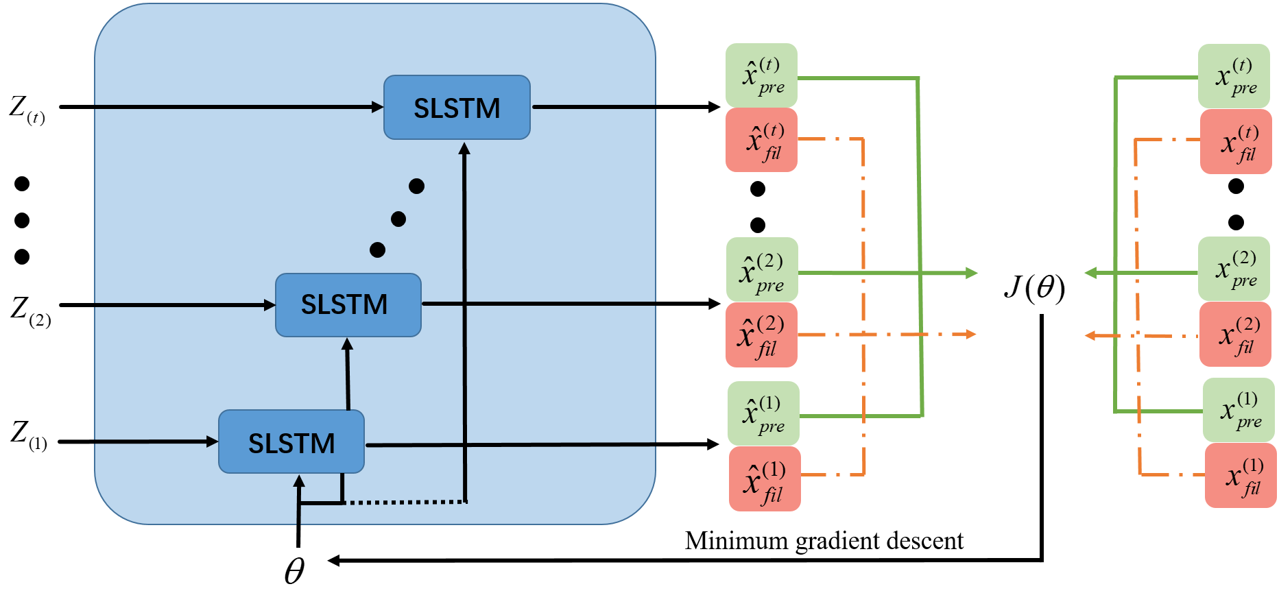
The neural network has strong robustness and fault tolerance. It can not only learn, organize and adapt itself so that the network can deal with uncertain systems but also fully approximate any complex nonlinear relationship. To enhance the estimation accuracy under multi-source data conditions, this paper proposes a deep fusion tracking framework based on a Stacked Long Short-Term Memory (SLSTM) network. This framework fuses multi-source trajectory observations (such as GPS measurements and auxiliary signals) to realize more accurate and robust trajectory tracking. The SLSTM model achieves trajectory fusion by learning the temporal dependencies and correlations from heterogeneous sensor data. It mimics the one-step prediction and one-step update steps in Bayesian and Kalman filtering. The network structure is illustrated in Figure 2. The input consists of fused trajectory data from multiple sources, and the output is the estimated trajectory. The network consists of the prediction module and the update module. The calculation Equation (11) of SLSTM is as follows:

\displaystyle\ C_{t-1}^{p},h_{t-1}^{p}=f_{h}^{p}({C_{t-1}},{h_{t-1}},{Z_{t-1}})

\displaystyle\ \hat{X}_{pre}^{(t|t-1)}=f_{o}^{p}(h_{t-1}^{p})

\displaystyle{C_{t}},{h_{t}}=f_{h}^{f}(C_{t-1}^{p},h_{t-1}^{p},\hat{X}_{pre}^{% (t|t-1)})

\displaystyle\ \hat{X}_{fil}^{(t|t)}=f_{o}^{f}({h_{t}})\

where $\hat{X}_{pre}^{(t|t-1)}$ is the predicted filter value of all measured values at the time $t-1$ , $\hat{X}_{fil}^{(t|t)}$ is the updated value at time . $f_{h}^{p}$ , $f_{o}^{p}$ and $f_{h}^{f}$ , correspond to the functions of the prediction filtering process and the update prediction process. Enter $Z_{t-1}$ , $h_{-1}$ , $C_{t-1}$ into the prediction part to get $C_{t-1}^{p}$ , $h_{t-1}$ , $\hat{X}_{pre}^{(t|t-1)}$ .Forecast results( $C_{t-1}^{p}$ , $h_{t-1}^{p}$ , $\hat{X}_{pre}^{(t|t-1)}$ ) enter the updated prediction part as the input to get the updated state. The hidden state is used as the input to enter the update part and get the updated state. Use the predicted status $\hat{X}_{pre}^{(t|t-1)}$ as input to the update section, estimate the target positions at time.

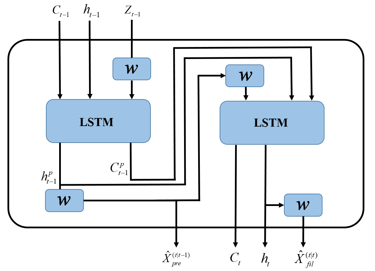
Figure 2 SLSTM Structure. The s are learnable parameters to make the dimensions of the input and output stay the same as those of the hidden states.

The first part of the network is the prediction part. LSTM is used to predict the input data $Z_{t-1}$ in one step, and the predicted value $\hat{X}_{pre}^{(t|t-1)}$ is used as the input to the second part of LSTM for updating to obtain the estimated value $\hat{X}_{fil}^{(t|t)}$ in one step. The first step of the network algorithm is prediction step (Equation (6) in Kalman filter). The second step of the network algorithm are updating step (Equation (7) in Kalman filter). Thus, the proposed method has a similar structure to the Kalman filter, consisting of a prediction equation and an update equation. This structural similarity provides several advantages, including the ability to leverage the well-established theoretical foundation of the Kalman filter and its well-known properties, such as optimality and convergence guarantees. The proposed method's similarity to the Kalman filter allows straightforward integration into pre-existing Kalman filter architectures, offering a more convenient and flexible framework for GPS-based tracking applications.

3.4 Training based on Bayesian variation

During training, the goal is not only to minimize the prediction and filtering error, but also to optimize the network to best fuse different sources of measurements. This is reflected in the cost function, which evaluates both the prediction and filtering accuracy across the fused data sequence. By leveraging fusion across multiple sensor modalities, the SLSTM model can better handle measurement noise, signal occlusion, and dynamic motion patterns. Therefore, the training process encourages the model to learn how to weight and utilize fused signals effectively.

Figure 3 shows the training structure of the SLSTM fusion network. LSTM requires a large amount of data to avoid overfitting. The input data shall be normalized to the maximum and minimum, and the data shall be mapped to the range of 0 $\sim$ 1 to accelerate the convergence of the training network.

One way to reduce the overfitting of neural networks when training the network is to use dropout, which is a regularization method. In each process, a part of hidden layer neurons is temporarily discarded by setting a certain probability to simplify the network to prevent overfitting and improve the network's generalization ability. After many experiments, the network works best when the dropout is set to 0.2.

After the network's training, the network, the output of the network is de-normalized to obtain the model's output value, and the network's parameters are optimized through the cost function. The cost function is nonconvex, and the calculation of the entire training data set is huge. Therefore, the minimum gradient descent algorithm is used to train the network to obtain parameters. The cost function of the network is Equation (12):

J(\theta)=\frac{1}{N}\sum{{}_{t=1}^{N}}[{(x_{fil}^{(t|t)}-\hat{x}_{fil}^{(t|t)% })^{2}}+\varepsilon{(x_{pre}^{(t|t-1)}-\hat{x}_{pre}^{(t|t-1)})^{2}}\

The superscript n represents the nth sequence in the training data set, which includes n sequences in total, $N$ is its length, and the weighting coefficient $\varepsilon$ that is a super parameter used to balance the error of filtering or estimation. If the sensor's accuracy is higher, it can be set to a value greater than 1.

The network cost consists of two parts, one is the result calculated from the input sequence through SLSTM, and the other is the actual value of GPS. The goal is to learn an actual trajectory network that can estimate close to the actual trajectory. Therefore, we minimize the mean square error between the filter, predicted, and actual states. The flow chart of training SLSTM to obtain its parameters is shown in Figure 3. The input value is $Z(t)$ , the prediction $\hat{x}_{pre}^{(t|t)}$ is obtained through the prediction module, and the filtering value $\hat{x}_{fil}^{(t)}$ is obtained through the filtering module. Therefore, the cost function is non convex. We use a gradient descent algorithm to optimize the parameters of SLSTM, namely $\theta$ . In order to overcome the problem of extensive calculation caused by large training data set when calculating gradient, it is only necessary to input a small batch of training samples to the network to update the parameters of each time step. The parameters of SLSTM are obtained by iterating the whole training dataset for some time until the cost function converges. In addition, optimization can be performed by randomly starting parameters to avoid local minima and find global minima with a higher probability. The network is a one-step prediction. It fully uses GPS data, trains the predicted value through the network, calculates the cost function with the measurement, and continuously optimizes the parameter $\theta$ .

Figure 3 Training architecture of the stacked LSTM fusion network. The input observation sequences

Z_{(t)}

are processed by the SLSTM blocks to generate predicted (

\hat{x}^{(i)}{pre}

) and filtered (

\hat{x}^{(i)}{fil}

) trajectories. These outputs are compared with ground-truth values to compute the cost function

J(\theta)

, which is minimized using gradient descent to optimize network parameters

\theta

Based on the above analysis, the optimization process of the SLSTM model is as follows:

Algorithm 1 Stacking LSTM Fusion Network Optimization Process

Step 1: Input multi-source GPS information, preprocess maximum and minimum normalized data for each track information, and set network parameters, drop=0.2, hidden_dim=32.
Step 2: Given a total of m samples for each batch: D( $Z_{t-1}$ ,X), where $Z$ represents the network input data, $x_{fil}^{(t)}$ represents the expected output of the network, and the network output is $x_{fil}^{(t)}$ .
Step 3: Use variational inference to sample the network weight and bias $N$ times and calculate the average loss: $J(\theta)=\frac{1}{N}\sum_{t=1}^{N}\left[(x_{fil}^{(t|t)}-\hat{x}_{fil}^{(t|t)% })^{2}+\varepsilon(x_{pre}^{(t|t-1)}-\hat{x}_{pre}^{(t|t-1)})^{2}\right]$
Step 4: Use the Adam optimizer according to loss to update the weight and parameters: $\theta$ .
Step 5: Repeat steps 2 to 4 for network convergence until the loss no longer declines.
Step 6: Use the test set to evaluate the trained network model.

4. Experiment and Result

4.1 Dataset

In this study, we simulated GPS trajectory with a total of 4,200 trajectories, which was equipped with pink noise to simulate measurement noise. To evaluate the performance of our proposed model, we split the entire data set into training and testing sets, with 80% of the data being used for model training, and the remaining 20% being reserved for model evaluation.

4.2 Experimental process and evaluation index

We built a deep learning model based on the open-source Python deep learning framework. All experiments were run on the PC of CPUAMD Ryzen 7 5800HCPU for several times, and the optimal super parameters were selected. The Adam optimization algorithm optimizes the deep learning model, and the optimized learning rate is 0.01; The data size of the input network is 32 tracks and all position information, and each iteration is 300 times.

This experiment uses four evaluation indicators to evaluate the experimental results: root means square error RMSE, mean absolute error MAE, mean square error MSE, and Pearson correlation coefficient $R^{2}$ . The four evaluation indicators can measure the gap between the estimated value given by the model and the actual value and evaluate the model's performance. The smaller the value of RMSE, MAE, and MSE, the smaller the difference between the estimated value and the actual value given by the model. The larger the value of R, the better the fitting ability of the model. The calculation Equations (13) - (16) of the four evaluation indicators are as follows:

RMSE = \sqrt{\frac{1}{N} \cdot \sum_{t = 1}^{N} {(x_{fil}^{(t | t)} - {\hat{x}}_{fil}^{(t | t)})}^{2}}

MAE{\rm{=}}\frac{1}{N}\sum\limits_{t=1}^{N}{\left|{(x_{fil}^{(t|t)}-\hat{x}_{% fil}^{(t|t)})}\right|}

MSE=\frac{1}{N}\sum\limits_{t=1}^{N}{{{(x_{fil}^{(t|t)}-\hat{x}_{fil}^{(t|t)})% }^{2}}}\

R^{2} = \frac{\sum_{t = 1}^{N} (x_{fil}^{(t | t)} - {\bar{x}}_{fil}^{(t | t)}) ({\hat{x}}_{fil}^{(t | t)} - {\bar{\hat{x}}}_{fil}^{(t | t)})}{\sqrt{\sum_{t = 1}^{N} {(x_{fil}^{(t | t)} - {\bar{x}}_{fil}^{(t | t)})}^{2}} \cdot \sqrt{\sum_{t = 1}^{N} {({\hat{x}}_{fil}^{(t | t)} - {\bar{\hat{x}}}_{fil}^{(t | t)})}^{2}}}

where $N$ is the total amount of data, $x_{fil}^{(t|t)}$ is the actual value of the data, $\hat{x}_{fil}^{(t|t)}$ is the trajectory value estimated by the model, $\bar{\hat{x}}_{fil}^{(t|t)}$ is the average value of the actual value, and $\bar{x}_{fil}^{(t|t)}$ is the average value of the estimated value.

4.3 Test results

This paper compares five classical path estimation models, including CV [10], CA [11], Singer [12], the current statistical model [13], and the adaptive model [42]. The data set used in this experiment is the data set with pink noise on the trajectory of the simulation target. This paper estimates the GPS data (The east direction of GPS is represented by the x-axis, and the y-axis represents the north direction of GPS). The noise variance of the CA model and CV model in the movement process is set to 200, and the noise variance and maneuvering frequency of the Singer model is set to 200 and 1, respectively. The current statistical model is sensitive to the set parameters, so multiple groups of maneuvering frequencies are set: $\alpha$ =1/10, $\alpha$ =1/20, and $\alpha$ =1/50. The results of the GPS data comparison experiment are shown in Table 1.

Table 1 Effect comparison with the classical model.

Model	direction	RMSE	MAE	MSE	R
CV^[10]	X	2.982	1.586	8.893	0.996
CV^[10]	Y	2.449	1.499	5.998	0.996
CA^[11]	X	2.348	1.531	5.515	0.986
CA^[11]	Y	2.072	1.474	4.294	0.991
singer^[12]	X	2.788	1.556	7.776	0.994
singer^[12]	Y	2.326	1.479	5.411	0.995
CS[^[13]	X	7.799	4.077	66.799	0.957
$\alpha$ =1/10	Y	6.683	4.128	48.954	0.964
CS^[14]	X	7.171	3.659	51.433	0.966
$\alpha$ =1/20	Y	6.139	3.653	37.694	0.971
CS^[15]	X	7.803	3.891	60.891	0.961
$\alpha$ =1/50	Y	6.695	3.957	44.831	0.966
Adaptive^[42]	X	11.556	6.790	133.563	0.949
Adaptive^[42]	Y	5.866	4.054	34.413	0.975
LSTM^[15]	X	2.452	1.786	6.016	0.978
LSTM^[15]	Y	2.246	1.697	5.048	0.983
SLSTM	X	1.916	1.499	3.673	0.997
SLSTM	Y	1.716	1.316	2.946	0.998

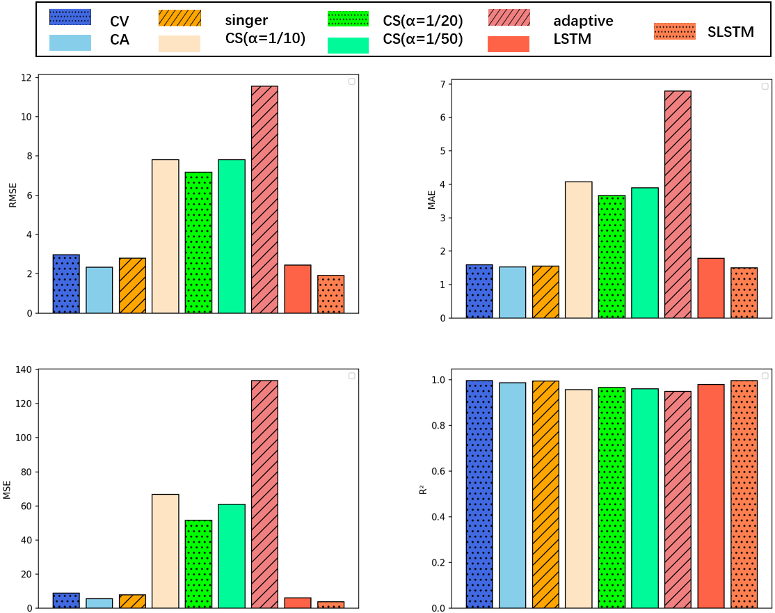
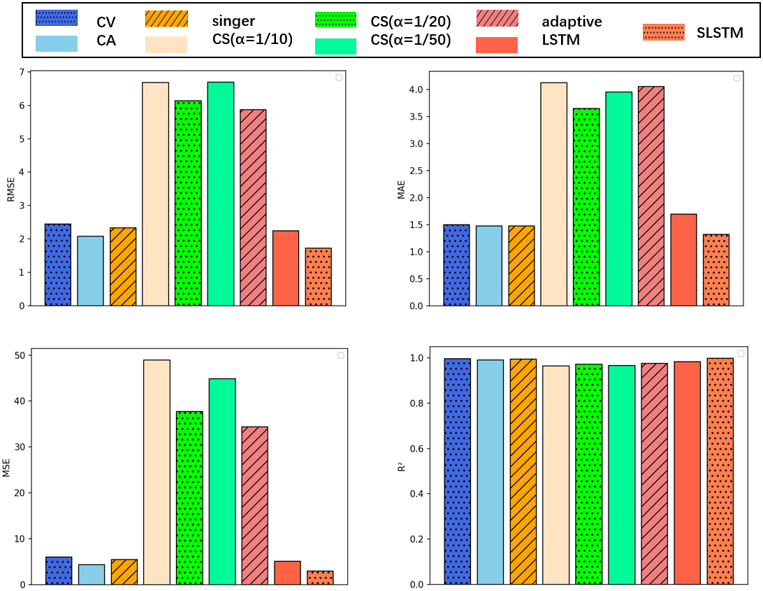
Figure 4 Comparison of fitting effects of X-coordinate.

Figure 5 Comparison of the fitting result of Y-coordinate.

The comparison results in Table 1 and Figures 4 - 10 show that the method proposed in this paper has improved the estimation accuracy compared with the classical and deep learning methods. Among them, the estimation result of the decoupled X coordinate is 18.3% higher than that of the model CA with the best result in the classical estimation method and 21.86% higher than that of the LSTM model; Compared with the best CA model in the classical model, the estimation result of the decoupled Y coordinate improves the precision by 17.19% and 23.6% compared with the LSTM model. Kalman algorithm is mainly aimed at the linear system, which requires the system and measurement noise to be a Gaussian model; UKF, EKF, and CKF can estimate the nonlinear system, but the noise is still required to be Gaussian noise; CV and CA models regard the acceleration and derivative of acceleration of maneuvering target as zero mean Gaussian noise, Singer model models the maneuvering target and acceleration as exponential autocorrelation zero mean colored noise, and the assumption of zero mean is unreasonable for describing the moving state of maneuvering target in real situations. The data set with pink noise is more in line with the actual project. The neural network can fit complex nonlinear data. The complex pink noise in the training data can be modeled in the network, which can realize the estimation of the data with pink noise. Figures 6 - 10 shows the estimation results based on CV, CA, CS, and Singer maneuver models, and the data-driven estimation method based on LSTM). It can be seen that the SLSTM network proposed in this paper has the best effect in fitting the actual position of moving targets. This is because SLSTM has a two-layer recursive structure. By learning the dynamic characteristics of the reference trajectory, the model information can be embedded into the deep learning network. Moreover, compared with the LSTM network model, the stacked serial dual LSTM structure proposed in this paper can obtain the characteristics of complex uncertain motion patterns, better express the mapping between the measured value and the actual value of the target, and thus get better trajectory estimation performance.

Figure 6 Comparison with estimation by Kalman Filters with CV model.

Figure 7 Comparison with estimation by Kalman Filters with CA model.

Figure 8 Comparison with estimation by Kalman Filters with CS model.

Figure 9 Comparison with estimation by Kalman Filters with Singer model.

Figure 10 Comparison with estimation by Kalman Filters with LSTM model.

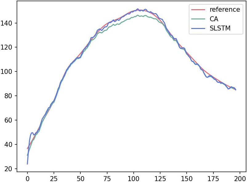
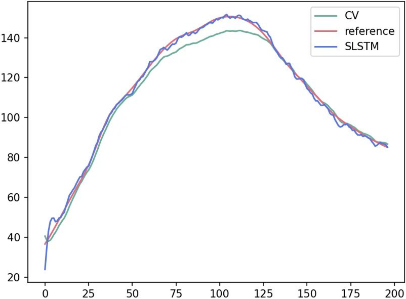
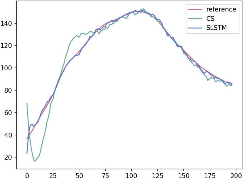
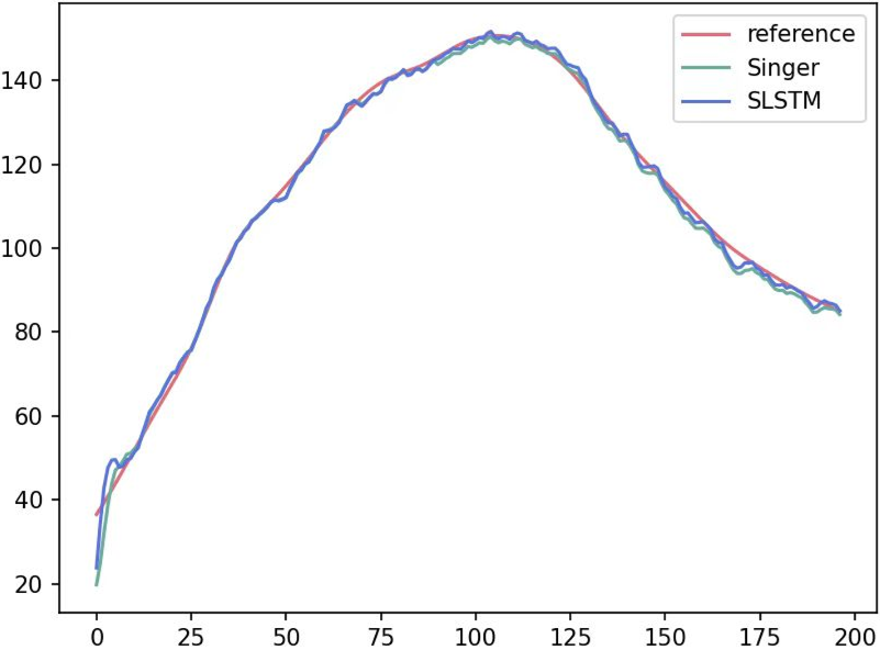
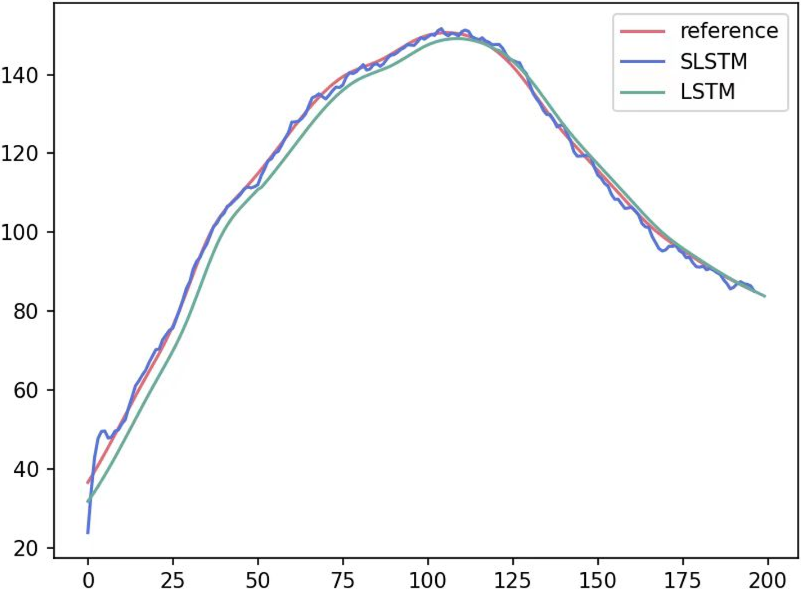
Figures 6 - 10 clearly demonstrate that SLSTM is compared with CV, CA, CS, the Singer model, and LSTM networks, respectively. Our experimental results indicate that SLSTM can more accurately fit various motion trajectories when the moving target is uncertain, outperforming both Kalman estimation based on the maneuver model and LSTM estimation.

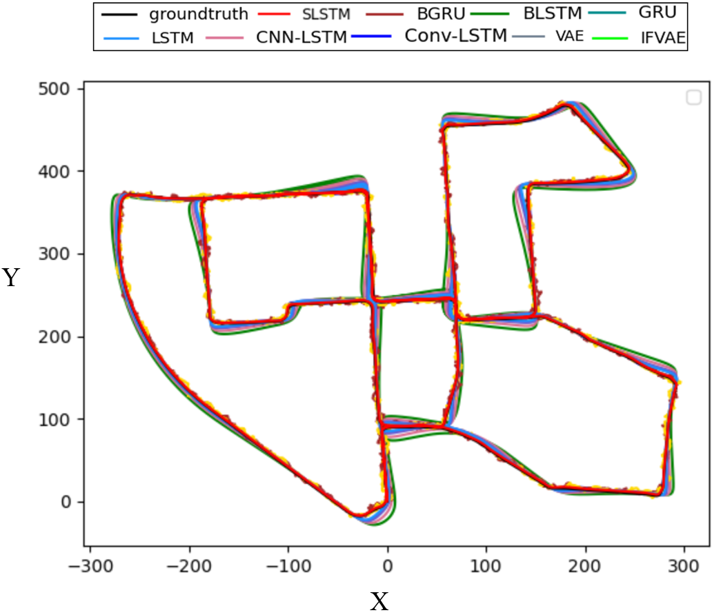
The dataset comprises 9,080 positional data points, representing the displacement information along the X and Y axes relative to the origin. This dataset is employed to compare eight distinct neural network models. For the neural network estimation experiments, each model is configured with a learning rate of 0.001, trained over 100 epochs, with a batch size of 20. The neural networks are designed with 2 layers and each hidden layer contains 24 neurons, with all data undergoing normalization. The variational autoencoder's encoding and decoding layers are each set to a single layer. The inverse autoregressive flow is configured with 5 layers, while the planar flow is set to 3 layers. As illustrated in Figure 11, the results of each model can be observed.

Figure 11 Comparison of different neural network models.

Table 2 Performance metrics for various neural network models.

Model	RMSE	MAE	MAPE	SMAPE	R
GRU	19.531	19.014	18.631	36.442	0.986
LSTM	26.753	25.945	24.322	35.273	0.935
BGRU	8.781	7.577	16.373	26.414	0.981
BLSTM	10.394	9.353	18.614	28.675	0.943
CNN-lstm	23.195	27.894	26.541	30.292	0.934
Conv-lstm	33.765	37.172	32.075	39.161	0.916
VAE	18.051	26.167	27.941	35.013	0.988
IFVAE	10.234	16.719	15.421	10.054	0.959
SLSTM	6.331	4.293	5.371	6.374	0.9991

As illustrated in Table 2, a thorough analysis of the performance metrics clearly indicates that the model proposed in this paper outperforms other network models across various performance indicators. Specifically, its RMSE, MAE, MAPE, and SMAPE values are all lower than those of other neural network models, signifying a smaller margin of error. Additionally, its R-value surpasses that of alternative models, demonstrating a higher degree of accuracy in fitting the reference.

5. Conclusion

Given the difficulty in modeling colored noise in the classical estimation methods and in matching the target motion model with the classical estimation methods, this paper proposes a short - and long-term neural network based on Bayesian filtering. It proposes a data-driven end-to-end state estimation method. The main contributions of this paper are as follows: design a stacked short and long-term fusion neural network, and estimate the target trajectory through recursive modules, SLSTM estimates the state of moving targets from noisy observation data, makes full use of the GPS data of moving targets, realizes one-step prediction, and trains the nonlinear relationship of different trajectories through neural networks, which can overcome the limitation of the estimation accuracy of traditional trajectory estimation methods. Compare with the X coordinate of the decoupled data, the accuracy of this method is 18.3% higher than that of the classical estimation method and 21.86% higher than that of LSTM; Compared with the Y coordinate of the decoupled data, the precision of this method is 17.19% higher than that of the classical estimation method. Compared with LSTM, the accuracy of this method is 23.6% higher. The experimental results show that this method is superior to the classical estimation and neural network methods. In future work, we will consider not only GPS information but also IMU information to further improves the model prediction accuracy.

Data Availability Statement

Data will be made available on request.

Funding

This work was supported without any funding.

Conflicts of Interest

The authors declare no conflicts of interest.

Ethical Approval and Consent to Participate

Not applicable.

References

Mathiassen, K., Hanssen, L., & Hallingstad, O. (2010, September). A low cost navigation unit for positioning of personnel after loss of GPS position. In 2010 international conference on indoor positioning and indoor navigation (pp. 1-10). IEEE.
CrossRef Google Scholar
Bar-Shalom, Y., Li, X. R., & Kirubarajan, T. (2004). Estimation with applications to tracking and navigation: theory algorithms and software. John Wiley & Sons.
Google Scholar
Julier, S. J., & Uhlmann, J. K. (1997, July). New extension of the Kalman filter to nonlinear systems. In Signal processing, sensor fusion, and target recognition VI (Vol. 3068, pp. 182-193). Spie.
CrossRef Google Scholar
Julier, S., Uhlmann, J., & Durrant-Whyte, H. F. (2000). A new method for the nonlinear transformation of means and covariances in filters and estimators. IEEE Transactions on automatic control, 45(3), 477-482.
CrossRef Google Scholar
Julier, S. J., & Uhlmann, J. K. (2004). Unscented filtering and nonlinear estimation. Proceedings of the IEEE, 92(3), 401-422.
CrossRef Google Scholar
Arasaratnam, I., & Haykin, S. (2009). Cubature kalman filters. IEEE Transactions on automatic control, 54(6), 1254-1269.
CrossRef Google Scholar
Li, P., Yu, J., Wan, M., Huang, J., & Huang, J. (2009, September). The augmented form of cubature Kalman filter and quadrature Kalman filter for additive noise. In 2009 IEEE Youth Conference on Information, Computing and Telecommunication (pp. 295-298). IEEE.
CrossRef Google Scholar
Chen, Y., Xie, X., Yu, B., Li, Y., & Lin, K. (2021). Multitarget vehicle tracking and motion state estimation using a novel driving environment perception system of intelligent vehicles. Journal of advanced transportation, 2021(1), 6251399.
CrossRef Google Scholar
Eltoukhy, M., Ahmad, M. O., & Swamy, M. N. S. (2020). An adaptive turn rate estimation for tracking a maneuvering target. IEEE Access, 8, 94176-94189.
CrossRef Google Scholar
Wang, L., & Zhou, G. (2021). Pseudo-spectrum based track-before-detect for weak maneuvering targets in range-Doppler plane. IEEE Transactions on Vehicular Technology, 70(4), 3043-3058.
CrossRef Google Scholar
Jia, S., Zhang, Y., & Wang, G. (2017). Highly maneuvering target tracking using multi-parameter fusion Singer model. Journal of Systems Engineering and Electronics, 28(5), 841-850.
CrossRef Google Scholar
Zhenkai, X., Fanying, L., & Lei, Z. (2018). Study on Maneuvering Target On-axis Tracking Algorithm of Modified Current Statistical Model. In MATEC Web of Conferences (Vol. 160, p. 02008). EDP Sciences.
CrossRef Google Scholar
Bar-Shalom, Y., & Blair, W. D. (1992). Multitarget-multisensor tracking: applications and advances. chapter 2.
Google Scholar
Lin, H. J., & Atherton, D. P. (1993, May). Investigation of IMM tracking algorithm for the maneuvering target tracking. In Proceedings. The First IEEE Regional Conference on Aerospace Control Systems, (pp. 113-117). IEEE.
CrossRef Google Scholar
Hochreiter, S., & Schmidhuber, J. (1997). Long short-term memory. Neural computation, 9(8), 1735-1780.
CrossRef Google Scholar
Chen, C., Zhao, P., Lu, C. X., Wang, W., Markham, A., & Trigoni, N. (2020). Deep-learning-based pedestrian inertial navigation: Methods, data set, and on-device inference. IEEE Internet of Things Journal, 7(5), 4431-4441.
CrossRef Google Scholar
Wang, B., Chen, C., Lu, C. X., Zhao, P., Trigoni, N., & Markham, A. (2020, April). Atloc: Attention guided camera localization. In Proceedings of the AAAI Conference on Artificial Intelligence (Vol. 34, No. 06, pp. 10393-10401).
CrossRef Google Scholar
Wang, S., Clark, R., Wen, H., & Trigoni, N. (2017, May). Deepvo: Towards end-to-end visual odometry with deep recurrent convolutional neural networks. In 2017 IEEE international conference on robotics and automation (ICRA) (pp. 2043-2050). IEEE.
CrossRef Google Scholar
Yang, Z., Tang, R., Bao, J., Lu, J., & Zhang, Z. (2020). A real-time trajectory prediction method of small-scale quadrotors based on GPS data and neural network. Sensors, 20(24), 7061.
CrossRef Google Scholar
Quan, Y., Lau, L., Roberts, G. W., Meng, X., & Zhang, C. (2018). Convolutional neural network based multipath detection method for static and kinematic GPS high precision positioning. Remote Sensing, 10(12), 2052.
CrossRef Google Scholar
Markos, C., James, J. Q., & Da Xu, R. Y. (2021, May). Capturing uncertainty in unsupervised GPS trajectory segmentation using Bayesian deep learning. In Proceedings of the AAAI Conference on Artificial Intelligence (Vol. 35, No. 1, pp. 390-398).
CrossRef Google Scholar
Nagui, N., Attallah, O., Zaghloul, M. S., & Morsi, I. (2021). Improved GPS/IMU loosely coupled integration scheme using two kalman filter-based cascaded stages. Arabian Journal for Science and Engineering, 46, 1345-1367.
CrossRef Google Scholar
Sun, Y., Xie, J., Guo, J., Wang, H., & Zhao, Y. (2014, December). A modified marginalized Kalman filter for maneuvering target tracking. In Proceedings of 2nd International Conference on Information Technology and Electronic Commerce (pp. 107-111). IEEE.
CrossRef Google Scholar
Huang, Y., Zhang, Y., Shi, P., & Chambers, J. (2020). Variational adaptive Kalman filter with Gaussian-inverse-Wishart mixture distribution. IEEE Transactions on Automatic Control, 66(4), 1786-1793.
CrossRef Google Scholar
Chang, Y., Wang, Y., Shen, Y., & Ji, C. (2021). A new fuzzy strong tracking cubature Kalman filter for INS/GNSS. GPS Solutions, 25(3), 120. https://link.springer.com/article/10.1007/s10291-021-01148-5
Google Scholar
Xiong, S. S., & Zhou, Z. Y. (2003). Neural filtering of colored noise based on Kalman filter structure. IEEE Transactions on Instrumentation and Measurement, 52(3), 742-747.
CrossRef Google Scholar
Morales, E. F., Murrieta-Cid, R., Becerra, I., & Esquivel-Basaldua, M. A. (2021). A survey on deep learning and deep reinforcement learning in robotics with a tutorial on deep reinforcement learning. Intelligent Service Robotics, 14(5), 773-805.
CrossRef Google Scholar
Yeo, K., & Melnyk, I. (2019). Deep learning algorithm for data-driven simulation of noisy dynamical system. Journal of Computational Physics, 376, 1212-1231.
CrossRef Google Scholar
Liu, J., Wang, Z., & Xu, M. (2020). DeepMTT: A deep learning maneuvering target-tracking algorithm based on bidirectional LSTM network. Information Fusion, 53, 289-304.
CrossRef Google Scholar
Zhang, J., Wu, Y., & Jiao, S. (2021, November). Research on trajectory tracking algorithm based on LSTM-UKF. In 2021 7th IEEE International Conference on Network Intelligence and Digital Content (IC-NIDC) (pp. 61-65). IEEE.
CrossRef Google Scholar
Li, S., Hu, C., Wang, R., Zhou, C., & Yang, J. (2019, December). A maneuvering tracking method based on LSTM and CS model. In 2019 IEEE International Conference on Signal, Information and Data Processing (ICSIDP) (pp. 1-4). IEEE.
CrossRef Google Scholar
Yaqi, C., You, H. E., Tiantian, T. A. N. G., & Yu, L. I. U. (2022). A new target tracking filter based on deep learning. Chinese Journal of Aeronautics, 35(5), 11-24.
CrossRef Google Scholar
Vedula, K., Weiss, M. L., Paffenroth, R. C., Uzarski, J. R., & Brown, D. R. (2020, November). Maneuvering target tracking using the autoencoder-interacting multiple model filter. In 2020 54th Asilomar Conference on Signals, Systems, and Computers (pp. 1512-1517). IEEE.
CrossRef Google Scholar
Giuliari, F., Hasan, I., Cristani, M., & Galasso, F. (2021, January). Transformer networks for trajectory forecasting. In 2020 25th international conference on pattern recognition (ICPR) (pp. 10335-10342). IEEE.
CrossRef Google Scholar
Hui, B., Yan, D., Chen, H., & Ku, W. S. (2021, August). Trajnet: A trajectory-based deep learning model for traffic prediction. In Proceedings of the 27th ACM SIGKDD Conference on Knowledge Discovery & Data Mining (pp. 716-724).
CrossRef Google Scholar
James, J. Q. (2020). Travel mode identification with GPS trajectories using wavelet transform and deep learning. IEEE Transactions on Intelligent Transportation Systems, 22(2), 1093-1103.
CrossRef Google Scholar
Liu, J., & Guo, G. (2021). Vehicle localization during GPS outages with extended Kalman filter and deep learning. IEEE Transactions on Instrumentation and Measurement, 70, 1-10.
CrossRef Google Scholar
Moradi, N., Nezhadshahbodaghi, M., & Mosavi, M. R. (2023). GPS signal acquisition based on deep convolutional neural network and post-correlation methods. GPS Solutions, 27(3), 132.
CrossRef Google Scholar
Taghizadeh, S., & Safabakhsh, R. (2023). An integrated INS/GNSS system with an attention-based hierarchical LSTM during GNSS outage. GPS Solutions, 27(2), 71.
CrossRef Google Scholar
He, S., Liu, J., Zhu, X., Dai, Z., & Li, D. (2023). Research on modeling and predicting of BDS-3 satellite clock bias using the LSTM neural network model. GPS Solutions, 27(3), 108.
CrossRef Google Scholar
Orouji, N., & Mosavi, M. R. (2021). A multi-layer perceptron neural network to mitigate the interference of time synchronization attacks in stationary GPS receivers. GPS solutions, 25, 1-15.
CrossRef Google Scholar
Venkataraman, V., Fan, G., Havlicek, J. P., Fan, X., Zhai, Y., & Yeary, M. B. (2012). Adaptive kalman filtering for histogram-based appearance learning in infrared imagery. IEEE transactions on image processing, 21(11), 4622-4635.
CrossRef Google Scholar

Cite This Article

APA Style

Jin, X., Liu, S., Kong, J., Bai, Y., Su, T., & Ma, H. (2024). GPS Tracking Based on Stacked-Serial LSTM Network. Chinese Journal of Information Fusion, 1(1), 50–62. https://doi.org/10.62762/CJIF.2024.361889

Export Citation

RIS Format

Compatible with EndNote, Zotero, Mendeley, and other reference managers

RIS format data for reference managers

TY  - JOUR
AU  - Jin, Xuebo
AU  - Liu, Songzheng
AU  - Kong, Jianlei
AU  - Bai, Yuting
AU  - Su, Tingli
AU  - Ma, Huijun
PY  - 2024
DA  - 2024/06/08
TI  - GPS Tracking Based on Stacked-Serial LSTM Network
JO  - Chinese Journal of Information Fusion
T2  - Chinese Journal of Information Fusion
JF  - Chinese Journal of Information Fusion
VL  - 1
IS  - 1
SP  - 50
EP  - 62
DO  - 10.62762/CJIF.2024.361889
UR  - https://www.icck.org/article/abs/CJIF.2024.361889
KW  - trajectory estimation
KW  - recurrent neural network
KW  - GPS
KW  - filtering algorithm
KW  - LSTM fusion networks
KW  - stacked serial structure
AB  - Maneuvering target tracking, as a core task in multi-sensor information fusion, is widely used in unmanned vehicles, missile navigation, and underwater ship localization, where real-time and robust state estimation is critical. Due to the uncertainty of the moving characteristics of maneuvering targets and the low sensor measurement accuracy, trajectory tracking has always been an open research problem and challenging work. This paper proposes a Bayesian-inspired stacked LSTM fusion network (SLSTM) for uncertain motion characteristics. The network consists of two LSTM fusion networks with stacked serial relationships, one of which is used to predict the movement dynamics, and the other is used to update the track's state. Compared with the classical Kalman filter based on the maneuver model, the method proposed here does not need to model the motion characteristics and sensor characteristics. It can achieve high-performance tracking by learning historical data dynamics and sensor characteristics. Experimental results show that this method can effectively improve the trajectory estimation performance when the target motion is unknown and uncertain.
SN  - 2998-3371
PB  - Institute of Central Computation and Knowledge
LA  - English
ER  -

BibTeX Format

Compatible with LaTeX, BibTeX, and other reference managers

BibTeX format data for LaTeX and reference managers

@article{Jin2024GPS,
  author = {Xuebo Jin and Songzheng Liu and Jianlei Kong and Yuting Bai and Tingli Su and Huijun Ma},
  title = {GPS Tracking Based on Stacked-Serial LSTM Network},
  journal = {Chinese Journal of Information Fusion},
  year = {2024},
  volume = {1},
  number = {1},
  pages = {50-62},
  doi = {10.62762/CJIF.2024.361889},
  url = {https://www.icck.org/article/abs/CJIF.2024.361889},
  abstract = {Maneuvering target tracking, as a core task in multi-sensor information fusion, is widely used in unmanned vehicles, missile navigation, and underwater ship localization, where real-time and robust state estimation is critical. Due to the uncertainty of the moving characteristics of maneuvering targets and the low sensor measurement accuracy, trajectory tracking has always been an open research problem and challenging work. This paper proposes a Bayesian-inspired stacked LSTM fusion network (SLSTM) for uncertain motion characteristics. The network consists of two LSTM fusion networks with stacked serial relationships, one of which is used to predict the movement dynamics, and the other is used to update the track's state. Compared with the classical Kalman filter based on the maneuver model, the method proposed here does not need to model the motion characteristics and sensor characteristics. It can achieve high-performance tracking by learning historical data dynamics and sensor characteristics. Experimental results show that this method can effectively improve the trajectory estimation performance when the target motion is unknown and uncertain.},
  keywords = {trajectory estimation, recurrent neural network, GPS, filtering algorithm, LSTM fusion networks, stacked serial structure},
  issn = {2998-3371},
  publisher = {Institute of Central Computation and Knowledge}
}

Article Metrics

Citations:

Google Scholar

Crossref

Scopus

Web of Science

Article Access Statistics:

PDF Downloads: 926

Publisher's Note

ICCK stays neutral with regard to jurisdictional claims in published maps and institutional affiliations.

Rights and Permissions

This article is an open access article distributed under the terms and conditions of the Creative Commons Attribution (CC BY) license.