Bifurcation and Stability Analysis of Transmission Dynamics of Ebola Virus Using Seirvh Model

Imtiaz Ahmad; Wali Ullah; Saeed Islam; Nigar Ali; Hazrat Younas; Muhammad Ijaz Khan

doi:10.62762/JAM.2025.550087

Abstract

This study presents a mathematical framework to analyze the transmission dynamics of the Ebola Virus Disease (EVD) using an extended SEIRVH model. The model incorporates vaccinated and hospitalized compartments, addressing critical factors such as vaccination efficacy, healthcare interventions, and natural disease progression. Differential equations describe the transitions between six population compartments. The study evaluates model stability and bifurcation through well-posedness, positivity, and boundedness analyzes, ensuring realistic and biologically valid solutions. The basic reproduction number, R0, derived from the next generation matrix, serves as a threshold for outbreak control. Local and global stability analyzes of disease-free and endemic equilibria reveal critical insights into epidemic thresholds and long-term dynamics. Furthermore, sensitivity analysis highlights key parameters that influence R0, emphasizing the importance of vaccination and hospitalization in mitigating EVD outbreaks. Numerical simulations validate theoretical findings, underscoring the model's utility in informing effective public health strategies, such as vaccination campaigns and hospitalization measures, for controlling EVD transmission. This research provides a robust analytical and computational tool for understanding and managing the spread of Ebola and similar infectious diseases.

Graphical Abstract

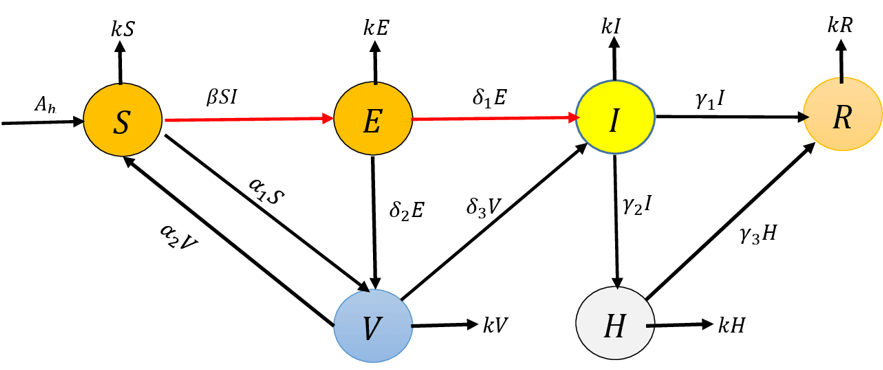
Bifurcation and Stability Analysis of Transmission Dynamics of Ebola Virus Using Seirvh Model

Click image to view fullscreen

Keywords

EBOLA stability analysis sensitivity analysis bifurcation analysis RK-4 method

1. Introduction

Ebola Virus Disease (EVD) is a highly virulent zoonotic illness caused by the Ebola virus, a member of the Filoviridae family. Clinically, EVD presents as an acute hemorrhagic fever syndrome, marked by high-grade fever, severe headache, vomiting, diarrhea, fatigue, and in many cases, internal and external bleeding, which can culminate in multi-organ failure [1, 10]. The disease was first identified in 1976 during simultaneous outbreaks in Sudan and Zaire (now the Democratic Republic of the Congo), with its name derived from the nearby Ebola River [1]. Since then, recurrent outbreaks, especially in Central and West Africa, have underscored its public health importance [2, 4].

The 2014–2016 West African epidemic, which severely impacted Guinea, Liberia, and Sierra Leone, was the largest on record in terms of geographic spread, morbidity, and mortality [4, 25]. EVD outbreaks typically exhibit case-fatality rates ranging from 25% to 90% [4, 10], emphasizing the critical need for timely detection, rapid intervention, and sustainable control strategies.

Transmission occurs primarily via direct contact with bodily fluids—such as blood, feces, or vomit—of symptomatic individuals or deceased patients. Indirect transmission via contaminated fomites has also been documented [3, 10]. In many of the most severely affected regions, weak diagnostic capacity, delayed response, and fragile healthcare infrastructure facilitate rapid amplification of the virus [4, 6].

Mathematical modeling has emerged as an indispensable tool in understanding infectious disease dynamics, particularly for EVD [3, 4, 6, 7, 10]. Compartmental models, especially those based on the classical SEIR (Susceptible–Exposed–Infectious–Recovered) structure, have been widely used to simulate epidemic trajectories, estimate key parameters such as the basic reproduction number $R_{0}$ , and assess the potential impact of public health interventions [16, 17, 21, 22].

In this study, we extend the standard SEIR framework by introducing two additional compartments: vaccinated ( $V$ ) and hospitalised ( $H$ ). The $V$ compartment reflects immunity through vaccination, while accounting for imperfect efficacy and waning protection [5, 25]. The $H$ compartment accounts for individuals receiving clinical care in isolation units, recognizing that hospitalisation reduces both mortality and transmission risk [13, 14]. Control measures, such as vaccination, hospitalisation, and awareness-based behavioral change, are incorporated explicitly to evaluate their respective effects on epidemic outcomes [11, 12, 14, 15].

The resulting model is a nonlinear system of ordinary differential equations (ODEs) with bilinear incidence, designed to capture both biological and policy-driven transitions. Below we describe the model formulation.

2. Model Formulation

To explore the transmission and control dynamics of EVD, we partition the total human population into six mutually exclusive epidemiological compartments:

$S(t)$ : Susceptible individuals.
$E(t)$ : Exposed (infected but not yet infectious) individuals.
$I(t)$ : Infectious individuals.
$V(t)$ : Vaccinated individuals.
$H(t)$ : Hospitalized individuals under clinical care.
$R(t)$ : Recovered individuals with acquired immunity.

2.1 Model Assumptions

The model is governed by the following assumptions, consistent with established EVD dynamics [3, 4, 5, 9]:

Recruitment into the susceptible population occurs at a constant rate $A_{h}$ .
Susceptible individuals are vaccinated at rate $\alpha_{1}$ ; vaccine-induced immunity wanes at rate $\alpha_{2}$ .
Susceptible individuals contract EVD via effective contact with infectious individuals at rate $\beta$ , modeled with a bilinear incidence term $\beta SI$ [3, 4].
Exposed individuals progress to the infectious class at rate $\delta_{1}$ , or are vaccinated (e.g., ring vaccination or post-exposure prophylaxis) at rate $\delta_{2}$ [5, 25].
Vaccinated individuals may still become infected due to vaccine failure at rate $\delta_{3}$ .
Infectious individuals recover at rate $\gamma_{1}$ or are hospitalized at rate $\gamma_{2}$ [13].
Hospitalized individuals recover or die (exit the compartment) at rate $\gamma_{3}$ .
All compartments are subject to a uniform natural mortality or removal rate $k$ .

Table 1 Descriptions of parameters used in the model.

Parameter	Interpretation
$A_{h}$	Recruitment rate into the susceptible class.
$\alpha_{1}$	Vaccination rate for susceptible individuals.
$\alpha_{2}$	Rate of waning immunity among vaccinated individuals.
$\beta$	Effective contact rate between susceptible and infectious individuals.
$\delta_{1}$	Progression rate from exposed to infectious.
$\delta_{2}$	Vaccination/intervention rate among exposed individuals.
$\delta_{3}$	Vaccine failure rate.
$\gamma_{1}$	Recovery rate of infectious individuals.
$\gamma_{2}$	Hospitalisation rate of infectious individuals.
$\gamma_{3}$	Recovery/mortality rate in hospitalized individuals.
$k$	Natural mortality/removal rate across all compartments.

2.2 Mathematical Model

The dynamics of the EVD transmission system are captured by the following set of nonlinear ODEs, with parameters defined in Table 1:

\begin{cases}\frac{dS}{dt}=A_{h}+\alpha_{2}V-(\alpha_{1}+k+\beta I)S,\\ \frac{dE}{dt}=\beta SI-(\delta_{1}+\delta_{2}+k)E,\\ \frac{dI}{dt}=\delta_{1}E+\delta_{3}V-(\gamma_{1}+\gamma_{2}+k)I,\\ \frac{dV}{dt}=\alpha_{1}S+\delta_{2}E-(\delta_{3}+\alpha_{2}+k)V,\\ \frac{dH}{dt}=\gamma_{2}I-(\gamma_{3}+k)H,\\ \frac{dR}{dt}=\gamma_{1}I+\gamma_{3}H-kR.\end{cases}

Subject to the following initial conditions:

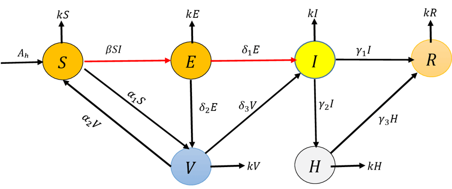
\displaystyle S(0)>0,\quad E(0)\geq 0,\quad I(0)\geq 0,

\displaystyle V(0)\geq 0,\quad H(0)\geq 0,\quad R(0)\geq 0.

Figure 1 presents the flow diagram representing the compartmental structure and transitions of the proposed model. Each parameter and transition is biologically motivated and derived from literature [3, 4, 10].

Figure 1 Flow diagram of the proposed Ebola virus transmission model.

3. Theoretical Analysis

3.1 Positivity of Solutions

.

Given non-negative initial conditions, all solutions of the system (1) remain non-negative for all $t\geq 0$ .

Proof..

We prove the non-negativity of each compartment in system (1) using contradiction and differential inequalities.Step 1: $S(t)\geq 0$ Suppose there exists a first time

t_{0}>0

such that

S(t_{0})=0

, with

S(t)>0

for

t<t_{0}

, and

S(t)<0

for some

t>t_{0}

. The governing equation is:

\frac{dS}{dt}=A_{h}+\alpha_{2}V-(\alpha_{1}+k+\beta I)S.

t=t_{0}

, since

S(t_{0})=0

, we have:

\left.\frac{dS}{dt}\right|_{t=t_{0}}=A_{h}+\alpha_{2}V(t_{0})\geq 0,

which contradicts

S(t)<0

for

t>t_{0}

. Thus,

S(t)\geq 0

for all

t\geq 0

. Step 2: $E(t)\geq 0$

\frac{dE}{dt}=\beta SI-(\delta_{1}+\delta_{2}+k)E.

E(t_{0})=0

, then

\frac{dE}{dt}=\beta SI\geq 0

, so

E(t)\geq 0

. Step 3: $I(t)\geq 0$

\frac{dI}{dt}=\delta_{1}E+\delta_{3}V-(\gamma_{1}+\gamma_{2}+k)I.

I(t_{0})=0

, then

\frac{dI}{dt}=\delta_{1}E+\delta_{3}V\geq 0

. Step 4: $V(t)\geq 0$

\frac{dV}{dt}=\alpha_{1}S+\delta_{2}E-(\delta_{3}+\alpha_{2}+k)V.

V(t_{0})=0

, then

\frac{dV}{dt}=\alpha_{1}S+\delta_{2}E\geq 0

. Step 5: $H(t)\geq 0$

\frac{dH}{dt}=\gamma_{2}I-(\gamma_{3}+k)H.

H(t_{0})=0

, then

\frac{dH}{dt}=\gamma_{2}I\geq 0

. Step 6: $R(t)\geq 0$

\frac{dR}{dt}=\gamma_{1}I+\gamma_{3}H-kR.

R(t_{0})=0

, then

\frac{dR}{dt}=\gamma_{1}I+\gamma_{3}H\geq 0

.Conclusion: All compartments remain non-negative for all

t\geq 0

. ∎

3.2 Disease-Free Equilibrium Point

The disease-free equilibrium (DFE) represents a state where no infection exists in the population:

(S^{*},E^{*},I^{*},V^{*},H^{*},R^{*})=\left(\frac{A_{h}}{\alpha_{1}+k},0,0,0,0% ,0\right).

The DFE is stable if the basic reproduction number $R_{0}\leq 1$ . When $R_{0}>1$ , the disease may invade and persist in the population.

3.3 Endemic Equilibrium Point

An endemic equilibrium refers to a state where the disease persists over time. The number of infections, recoveries, and deaths balance such that:

\displaystyle S^{*}=\frac{A_{h}-V^{*}}{\alpha_{1}+k+\beta I^{*}},

\displaystyle E^{*}=\frac{\beta S^{*}I^{*}}{\delta_{1}+\delta_{2}+k},

\displaystyle I^{*}=\frac{\delta_{1}E^{*}+\delta_{3}V^{*}}{\gamma_{1}+\gamma_{% 2}+k},

\displaystyle V^{*}=\frac{\alpha_{1}S^{*}+\delta_{2}E^{*}}{\delta_{3}+\alpha_{% 2}+k},

\displaystyle H^{*}=\frac{\gamma_{2}I^{*}}{\gamma_{3}+k},

\displaystyle R^{*}=\frac{\gamma_{1}I^{*}+\gamma_{3}H^{*}}{k}.

3.4 Model Analysis and Boundedness

Define the total human population as:

N(t)=S(t)+E(t)+I(t)+V(t)+H(t)+R(t).

Differentiating, we obtain:

\frac{dN}{dt}=A_{h}-kN(t).

Solving the differential equation yields:

N(t)=N(0)e^{-kt}+\frac{A_{h}}{k}(1-e^{-kt}).

Hence, as $t\to\infty$ , the population tends to:

\lim_{t\to\infty}N(t)=\frac{A_{h}}{k}.

.

The region

\Omega=\left\{(S,E,I,V,H,R)\in\mathbb{R}_{+}^{6}:N(t)\leq\frac{A_{h}}{k}\right\}

is positively invariant.

Proof..

From the total population dynamics:

\frac{dN}{dt}=A_{h}-kN,

with the integrating factor method, we obtain:

N(t)\geq N(0)e^{-kt}+\frac{A_{h}}{k}(1-e^{-kt}).

Therefore,

N(t)\to\frac{A_{h}}{k}

t\to\infty

, and solutions are bounded within region

\Omega

. Furthermore, since each component satisfies:

\begin{pmatrix}S(t)\\ E(t)\\ I(t)\\ V(t)\\ H(t)\\ R(t)\end{pmatrix}\in\mathbb{R}_{+}^{6},

the model is mathematically well-posed and epidemiologically meaningful. ∎

4. Basic Reproduction Number (R0)

The basic reproduction number, denoted as $R_{0}$ , is a critical threshold used to evaluate the potential for disease spread in a fully susceptible population. Specifically, $R_{0}$ represents the expected number of secondary infections produced by a single infectious individual introduced into a completely susceptible population. When $R_{0}<1$ , the disease cannot invade the population and will eventually die out. Conversely, if $R_{0}>1$ , the disease may cause an outbreak and persist in the population. Thus, understanding and computing $R_{0}$ is crucial for predicting the future dynamics of the disease and guiding effective control strategies.

Numerous studies have addressed the determination of $R_{0}$ for various epidemiological models [15, 16]. In this work, we compute $R_{0}$ for the proposed model (1) using the next-generation matrix method [17, 18]. The infection subsystem is isolated, and the matrices $F$ and $V$ are constructed in accordance with the formulation given in [8].

The infection subsystem of the model (1) is given by:

\begin{cases}\frac{dE}{dt}=\beta SI-(\delta_{1}+\delta_{2}+k)E,\\ \frac{dI}{dt}=\delta_{1}E+\delta_{3}V-(\gamma_{1}+\gamma_{2}+k)I,\\ \frac{dV}{dt}=\alpha_{1}S+\delta_{2}E-(\delta_{3}+\alpha_{2}+k)V.\end{cases}

The new infection matrix $F$ and its Jacobian at the disease-free equilibrium are:

F=\begin{pmatrix}\beta SI\\ 0\\ 0\end{pmatrix},\quad F^{*}=\begin{pmatrix}0&\beta S_{0}&0\\ 0&0&0\\ 0&0&0\end{pmatrix}.

The transition matrix $V$ is defined as:

V=\begin{pmatrix}(\delta_{1}+\delta_{2}+k)E\\ (\gamma_{1}+\gamma_{2}+k)I-\delta_{1}E-\delta_{3}V\\ (\delta_{3}+\alpha_{2}+k)V-\delta_{2}E\end{pmatrix}.

The inverse of the Jacobian of $V$ evaluated at the disease-free equilibrium is:

V^{*-1}=\begin{pmatrix}\delta_{1}+\delta_{2}+k&0&0\\ -\delta_{1}&\gamma_{1}+\gamma_{2}+k&-\delta_{3}\\ -\delta_{2}&0&\delta_{3}+\alpha_{2}+k\end{pmatrix}.

Multiplying $F^{*}$ and $V^{*-1}$ yields:

FV^{-1}=\begin{pmatrix}\frac{\beta S_{0}\delta_{1}}{(\delta_{1}+\delta_{2}+k)(% \gamma_{1}+\gamma_{2}+k)}&\frac{\beta S_{0}}{\gamma_{1}+\gamma_{2}+k}&0\\ 0&0&0\\ 0&0&0\end{pmatrix}.

The basic reproduction number $R_{0}$ is given by the spectral radius of $FV^{-1}$ :

R_{0}=\frac{\beta\delta_{1}A_{h}}{(\delta_{1}+\delta_{2}+k)(\gamma_{1}+\gamma_% {2}+k)(\alpha_{1}+k)}.

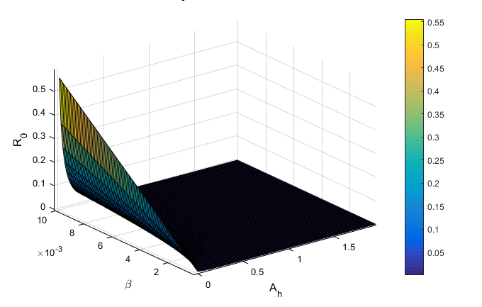
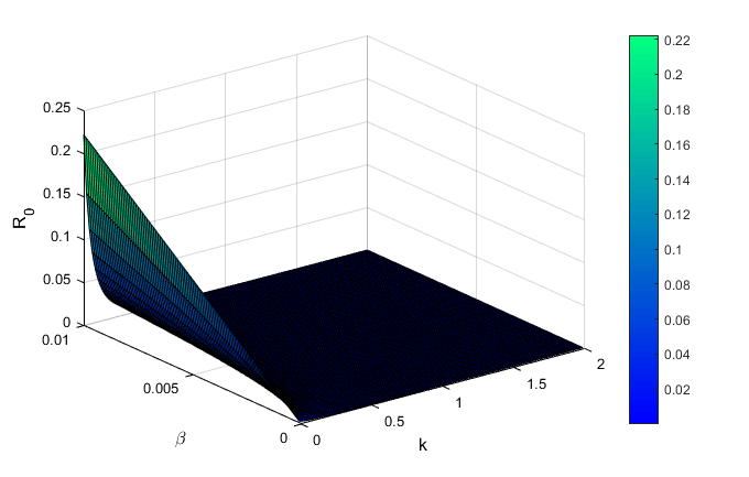
The effects of the parameters $\beta$ , $A_{h}$ , and $k$ on $R_{0}$ are illustrated in Figure 2, highlighting their influence on the potential for disease spread.

Figure 2 Effects of

\beta

A_{h}

, and

k

R_{0}

4.1 Local Stability of the Disease-Free Equilibrium

.

The disease-free equilibrium $E_{0}$ of system (1) is locally asymptotically stable if $R_{0}<1$ and unstable if $R_{0}>1$ .

Proof..

At the disease-free equilibrium point

E_{0}

, the Jacobian matrix of system (1) is:

JE_{0}=\begin{pmatrix}-(\alpha_{1}+k)&0&\beta S^{*}&\alpha_{2}&0&0\\ 0&-Z_{1}&\beta S^{*}&0&0&0\\ 0&\delta_{1}&-Z_{2}&\delta_{3}&0&0\\ \alpha_{1}&\delta_{2}&0&-(\delta_{3}+\alpha_{2}+k)&0&0\\ 0&0&\gamma_{2}&0&-(\gamma_{3}+k)&0\\ 0&0&\gamma_{1}&0&\gamma_{3}&-k\end{pmatrix},

where

Z_{1}=\delta_{1}+\delta_{2}+k

and

Z_{2}=\gamma_{1}+\gamma_{2}+k

. The eigenvalues of this matrix are:

\displaystyle\lambda_{1}=-(\alpha_{1}+k),\quad\lambda_{2}=-(\gamma_{1}+\gamma_% {2}+k),

\displaystyle\lambda_{3}=-k,\quad\lambda_{4}=-Z_{1},

\displaystyle\lambda_{5}=-Z_{1}Z_{2},\quad\lambda_{6}=-Z_{1}Z_{2}(\delta_{3}+% \alpha_{2}+k).

Since all eigenvalues are negative when

R_{0}<1

, the disease-free equilibrium is locally asymptotically stable by the Routh-Hurwitz criterion [21, 22, 24]. ∎

4.2 Global Stability of the Endemic Equilibrium

.

If $R_{0}>1$ , then the endemic equilibrium $E_{1}$ of system (1) is globally asymptotically stable in $\Omega$ .

Proof..

For

R_{0}>1

, the existence of a unique endemic equilibrium

E_{1}

is guaranteed. We consider the standard Lyapunov function [23]:

V(x)=\sum_{i=1}^{n}\frac{c_{i}}{2}(x_{i}-x_{i}^{*})^{2},

which, for our system, takes the form:

\displaystyle V(S,E,I,V,H,R)=\frac{1}{2}\left[(S-S^{*})+(E-E^{*})\right.

\displaystyle\left.+(I-I^{*})+(V-V^{*})+(H-H^{*})+(R-R^{*})\right]^{2}.

Differentiating (10) along solutions of system (1), and noting that:

\frac{d}{dt}(S+E+I+V+H+R)=-k(S+E+I+V+H+R),

we obtain:

\begin{aligned} \frac{dV}{dt}&=-k(S+E+I+V+H+R)\cdot\left[(S-S^{*})+(E-E^{*})% \right.\\ &\quad\left.+(I-I^{*})+(V-V^{*})+(H-H^{*})+(R-R^{*})\right].\end{aligned}

Clearly,

\frac{dV}{dt}\leq 0

, and equality holds if and only if the state variables equal their endemic equilibrium values. Hence, by LaSalle's Invariance Principle [23], the endemic equilibrium

E_{1}

is globally asymptotically stable in

\Omega

. ∎

4.3 Sensitivity Analysis of 𝑹𝟎

The sensitivity analysis of the basic reproduction number $R_{0}$ with respect to model parameters plays a crucial role in understanding the influence of each parameter on disease transmission, control, and treatment effectiveness, as demonstrated in similar infectious disease models [19]. This analysis identifies which parameters most significantly impact $R_{0}$ and thus should be prioritized in disease mitigation strategies.

We examine the sensitivity of $R_{0}$ in relation to the key parameters of the Ebola virus model (1). The sensitivity index of a parameter $\psi$ is computed using the normalized forward sensitivity index as proposed by Chitnis et al. [21], defined as:

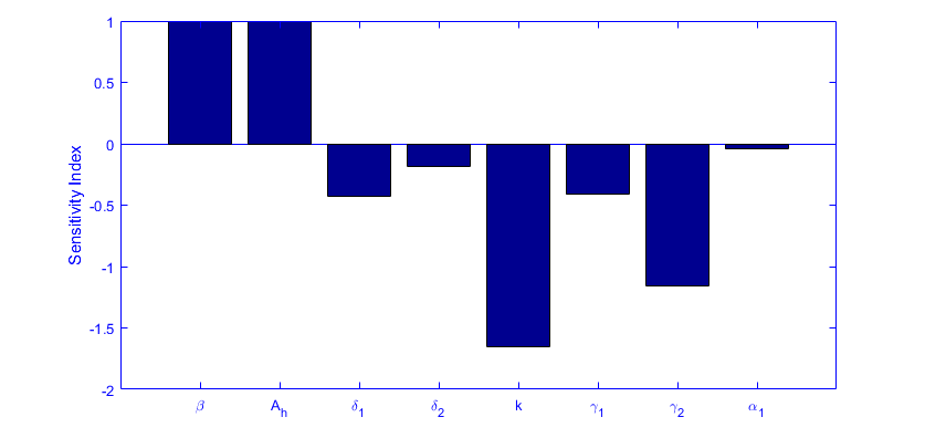
X_{\psi}^{R_{0}}=\frac{\partial R_{0}}{\partial\psi}\times\frac{\psi}{R_{0}}

The sensitivity indices for relevant model parameters are computed as follows, with their impacts illustrated in Figure 3:

\begin{aligned} X_{\beta}^{R_{0}}&=1,\quad X_{A_{h}}^{R_{0}}=1,\\ X_{\delta_{1}}^{R_{0}}&=-\frac{\delta_{1}}{\delta_{1}+\delta_{2}+k},\quad X_{% \delta_{2}}^{R_{0}}=-\frac{\delta_{2}}{\delta_{1}+\delta_{2}+k},\\ X_{k}^{R_{0}}&=-k\left(\frac{1}{\delta_{1}+\delta_{2}+k}+\frac{1}{\gamma_{1}+% \gamma_{2}+k}+\frac{1}{\alpha_{1}+k}\right),\\ X_{\gamma_{1}}^{R_{0}}&=-\gamma_{1}\left(\frac{(\delta_{1}+\delta_{2}+\gamma_{% 1})(\alpha_{1}+k)+(\gamma_{1}+\gamma_{2}+k)(\alpha_{1}+k)}{(\delta_{1}+\delta_% {2}+\gamma_{1})(\gamma_{1}+\gamma_{2}+k)(\alpha_{1}+k)}\right),\\ X_{\gamma_{2}}^{R_{0}}&=-\gamma_{2}\left(\frac{(\delta_{1}+\delta_{2}+\gamma_{% 1})(\alpha_{1}+k)+(\gamma_{1}+\gamma_{2}+k)(\delta_{1}+\delta_{2}+\gamma_{1})}% {(\delta_{1}+\delta_{2}+\gamma_{1})(\gamma_{1}+\gamma_{2}+k)(\alpha_{1}+k)}% \right),\\ X_{\alpha_{1}}^{R_{0}}&=-\alpha_{1}\cdot\frac{\beta A_{h}(\delta_{1}+\delta_{2% }+\gamma_{1})}{(\delta_{1}+\delta_{2}+\gamma_{1})^{2}(\gamma_{1}+\gamma_{2}+k)% ^{2}}\end{aligned}

Figure 3 Sensitivity indices of parameters influencing

R_{0}

5. Optimal Control System

Figure 4 Dynamics of EVD compartments with and without control interventions (

m_{1}

m_{2}

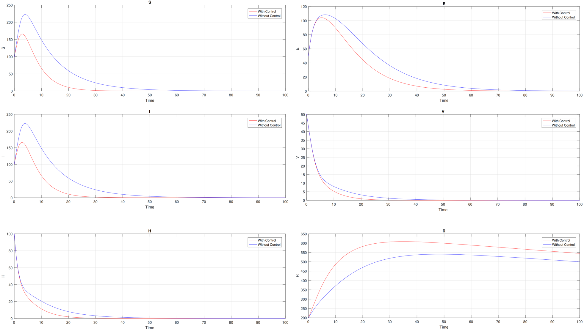
To further mitigate the Ebola Virus Disease (EVD), we expand the model (1) by incorporating two time-dependent control functions: $m_{1}(t)$ and $m_{2}(t)$ . Here, $m_{1}(t)$ represents enhanced diagnostic efforts for exposed individuals, while $m_{2}(t)$ captures the immediate treatment of infected individuals. The extended model is given by:

\displaystyle\frac{dS}{dt}=A_{h}+\alpha_{2}V-(\alpha_{1}+k)S-(1-m_{1})\beta IS,

\displaystyle\frac{dE}{dt}=(1-m_{1})\beta IS-(\delta_{1}+\delta_{2}+k)E,

\displaystyle\frac{dI}{dt}=\delta_{1}E+\delta_{3}V-(\gamma_{1}+m_{2}\gamma_{2}% +k)I,

\displaystyle\frac{dV}{dt}=\alpha_{1}S+\delta_{2}E-(\delta_{3}+\alpha_{2}+k)V,

\displaystyle\frac{dH}{dt}=m_{2}\gamma_{2}I-(\gamma_{3}+k)H,

\displaystyle\frac{dR}{dt}=\gamma_{1}I+\gamma_{3}H-kR.

The impact of these control measures on the dynamics of the EVD compartments is illustrated in Figure 4. The goal is to minimize the number of exposed and infected individuals while also minimizing the costs of the control measures. This is achieved via the following cost functional:

\displaystyle\mathcal{J}(m_{1},m_{2})=\int_{t_{0}}^{t_{f}}\left[\mathcal{B}_{1% }E+\mathcal{B}_{2}I\right]dt

\displaystyle\quad+\frac{1}{2}\left(\mathcal{B}_{3}m_{1}^{2}(t)+\mathcal{B}_{4% }m_{2}^{2}(t)\right),

subject to the admissible control set:

\mathcal{U}=\left\{m_{j}(t)\colon 0\leq m_{j}(t)\leq 1,\quad j=1,2,\quad t\in[% 0,t_{f}]\right\}.

5.1 Characterization of Optimal Control

Applying Pontryagin's Maximum Principle [23], a widely used approach in infectious disease control models [20], the Hamiltonian $\mathcal{H}$ for the system is given as:

\displaystyle\mathcal{H}=\mathcal{B}_{1}E+\mathcal{B}_{2}I+\frac{1}{2}\left(% \mathcal{B}_{3}m_{1}^{2}+\mathcal{B}_{4}m_{2}^{2}\right)

\displaystyle\quad+\sum_{i=1}^{6}\lambda_{i}\frac{dx_{i}}{dt},

where $\lambda_{i}$ are the adjoint variables corresponding to state variables $S, E, I, V, H,$ and $R$ .

The adjoint system is governed by:

\displaystyle\frac{d\lambda_{1}}{dt}=\lambda_{1}(\alpha_{1}+k)+(\lambda_{1}-% \lambda_{2})(1-m_{1})\beta I+\lambda_{4}\alpha_{1},

\displaystyle\frac{d\lambda_{2}}{dt}=-\mathcal{B}_{1}+(\delta_{1}+\delta_{2}+k% )\lambda_{2}-\lambda_{3}\delta_{1}-\lambda_{4}\delta_{2},

\displaystyle\frac{d\lambda_{3}}{dt}=-\mathcal{B}_{2}+(\lambda_{1}-\lambda_{2}% )(1-m_{1})\beta S

\displaystyle\quad+\lambda_{3}(\gamma_{1}+m_{2}\gamma_{2}+k)-\lambda_{5}m_{2}% \gamma_{2}-\lambda_{6}\gamma_{1},

\displaystyle\frac{d\lambda_{4}}{dt}=-\lambda_{1}\alpha_{1}-\lambda_{3}\delta_% {3}+\lambda_{4}(\delta_{2}+\alpha_{2}+k),

\displaystyle\frac{d\lambda_{5}}{dt}=\lambda_{5}(\gamma_{3}+k)-\lambda_{6}% \gamma_{3},

\displaystyle\frac{d\lambda_{6}}{dt}=\lambda_{6}k,

with transversality conditions:

\lambda_{i}(t_{f})=0,\quad\text{for }i=1,\dots,6.

The optimal controls are characterized by:

\displaystyle m_{1}^{*}(t)=\min\left(1,\max\left(0,\frac{(\lambda_{2}-\lambda_% {1})\beta IS}{\mathcal{B}_{3}}\right)\right),

\displaystyle m_{2}^{*}(t)=\min\left(1,\max\left(0,\frac{(\lambda_{3}-\lambda_% {5})\gamma_{2}I}{\mathcal{B}_{4}}\right)\right).

Combining the state system (1), the adjoint system (4), and the optimal controls (5), we obtain the full optimality system for simulation and control implementation.

5.2 Discussion

The relationship between the infection rate $\beta$ and the basic reproduction number $R_{0}$ is direct and proportional. An increase in $\beta$ leads to a corresponding increase in $R_{0}$ , indicating that transmission intensity escalates with higher infection rates. Therefore, reducing $\beta$ is essential for outbreak control. This can be achieved through interventions such as immunization, isolation, public health education, and hygiene improvements.

The sensitivity index of $\delta_{1}$ is negative, implying that an increase in $\delta_{1}$ reduces $R_{0}$ . A higher mortality rate in the first infectious class shortens the infectious period, thereby limiting disease transmission. Similarly, an increase in $\delta_{2}$ also lowers $R_{0}$ , underscoring the role of mortality in reducing the number of secondary infections.

For the recovery rate $k$ , its sensitivity index is also negative. Enhancing the recovery rate through medical treatment or supportive care diminishes the number of infectious individuals, hence reducing $R_{0}$ .

The transition parameters $\gamma_{1}$ and $\gamma_{2}$ represent movement between different risk groups or health statuses. Their negative sensitivity indices suggest that facilitating transitions (e.g., hospitalization or effective isolation) can mitigate disease spread.

Furthermore, the natural death rate $\alpha_{1}$ exhibits a negative sensitivity index. A higher $\alpha_{1}$ reduces the pool of susceptible individuals, thereby lowering the overall transmission potential.

6. Numerical Simulation

To analyze the impact of model parameters on the disease dynamics, we evaluate the sensitivity of the basic reproduction number $R_{0}$ using the normalized forward sensitivity index defined by Chitnis et al. [21], given by Equation (13).

\Gamma_{\theta}^{R_{0}}=\frac{\partial R_{0}}{\partial\theta}\cdot\frac{\theta% }{R_{0}},

where $\theta$ denotes a given model parameter. Sensitivity analysis helps identify key parameters for intervention strategies.

Figure 5 Dynamics of compartments

S, E, I, V, H,

and

R

Figure 6 Effect on Susceptible class.

Figure 7 Effect of hospitalization on susceptible population.

Figure 8 Effect on exposed class.

Figure 9 Effect on infectious class.

Figure 10 Effect on recovered class.

Figure 11 Vaccination impact on susceptible class.

Figure 12 Vaccination impact on exposed class.

Figure 13 Vaccination impact on infected class.

Figure 14 Vaccination impact on recovered class.

Figure 15 Hospitalized population under vaccination.

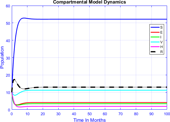
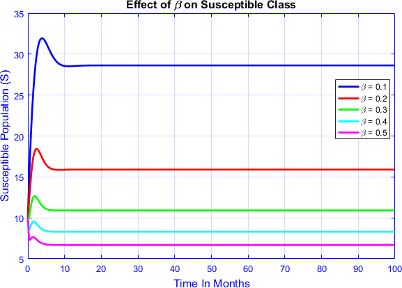
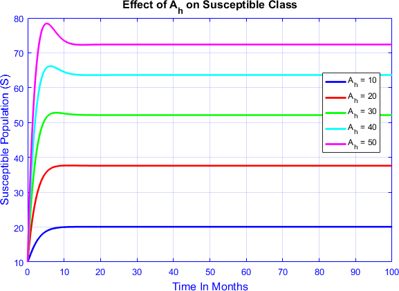
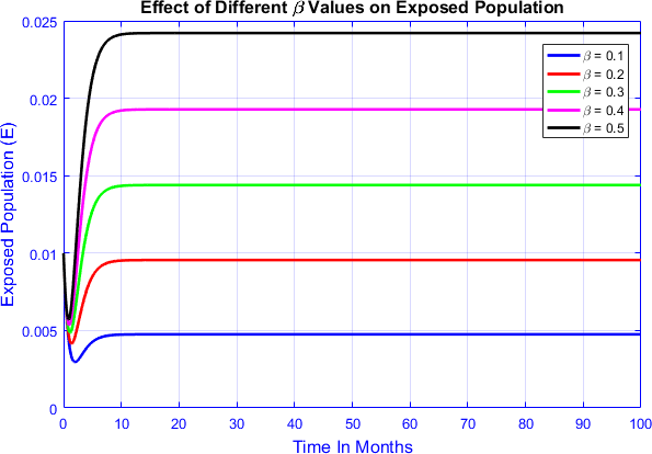
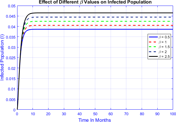
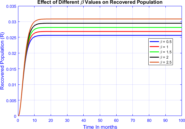
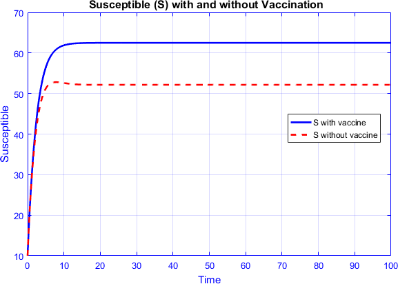
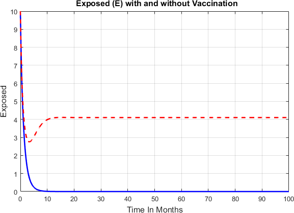
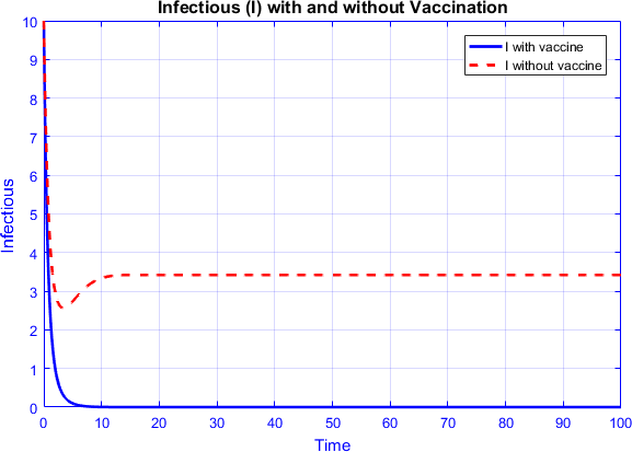
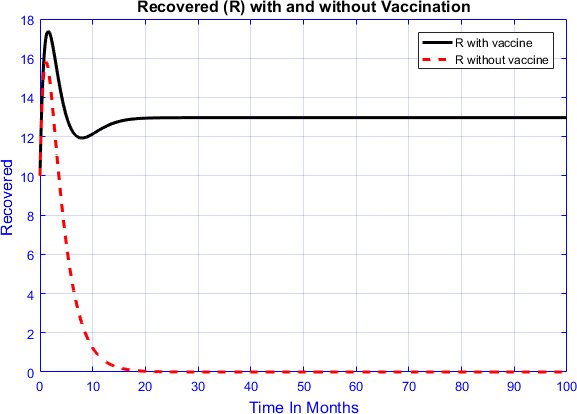
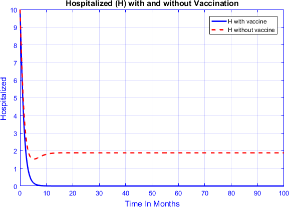
Figure 5 illustrates the time evolution of each compartment in the SEIRVH model. During simulations, a subset of parameters is varied while others remain constant to assess system response. When $\beta=0.003$ , we find that $R_{0}=0.9<1$ , and the disease-free equilibrium (DFE) is locally asymptotically stable.

Similarly, for $\beta=0.0006$ , $R_{0}=0.1499<1$ , the system also converges to the DFE. In contrast, when $\beta=0.006$ , resulting in $R_{0}=1.4990>1$ , the system approaches an endemic equilibrium, aligning with Theorem 4.1 and Theorem 4.2.

Figures 6–15 show that increasing $\beta$ accelerates the depletion of the susceptible population and intensifies the epidemic. A smaller $\beta$ (e.g., 0.1) leads to slower disease spread, while a higher $\beta$ (e.g., 0.5) results in rapid increases in exposed and infectious individuals.

Vaccination effects are evident in Figures 11–14. With vaccination, the susceptible, exposed, and infectious populations decline more quickly. The number of recovered individuals increases, indicating improved control over disease spread.

7. Conclusion Remarks

This study presents a comprehensive analytical and numerical investigation of the Ebola Virus Disease (EVD) through an extended SEIRVH model that incorporates vaccination and hospitalization. The model's well-posedness, positivity, and boundedness affirm its biological validity.

Using the next-generation matrix approach, we derived the basic reproduction number $R_{0}$ and assessed local and global stability for both disease-free and endemic equilibria. The Lyapunov function method confirms the global stability conditions, while sensitivity analysis reveals the most influential parameters on $R_{0}$ .

A backward bifurcation was identified using Center Manifold theory, emphasizing the challenge of achieving disease eradication even when $R_{0}<1$ . Optimal control analysis incorporating vaccination, therapy, and public awareness further illustrates effective mitigation strategies.

Numerical simulations validate the theoretical results and demonstrate the crucial role of reducing $\beta$ through public health interventions. Moreover, the Non-standard Finite Difference (NSFD) scheme outperformed the classical RK-4 method in simulating disease dynamics.

Overall, this model provides a robust tool for understanding and managing EVD outbreaks. It highlights the necessity of integrated strategies combining vaccination, hospitalization, and timely interventions, offering practical guidance for public health authorities to mitigate the devastating impacts of infectious diseases.

Data Availability Statement

Data will be made available on request.

Funding

This work was supported without any funding.

Conflicts of Interest

The authors declare no conflicts of interest.

Ethical Approval and Consent to Participate

Not applicable.

References

Piot, P., Sureau, P., Breman, G., Heymann, D., Kintoki, V., Masamba, M., & Mbuy, M. (1978). Clinical aspects of Ebola virus infection in Yambuku area, Zaire 1976. African Journal of Infectious Diseases, 210(96), 34–51.
Google Scholar
Chretien, J. P., Riley, S., & George, D. B. (2015). Mathematical modeling of the West Africa Ebola epidemic. Elife, 4, e09186.
CrossRef Google Scholar
Durojaye, M., & Ajie, J. (2017). Mathematical model of the spread and control of Ebola virus disease. Applied Mathematics, 7, 23–31.
Google Scholar
Mbah, G. C., Sunday, O. I., Ojoma, A. Q., Christopher, A., & Chukwudi, O. (2023). Mathematical modelling approach of the study of Ebola virus disease transmission dynamics in a developing country. African Journal of Infectious Diseases, 17(1), 10–26.
Google Scholar
Tadmon, C., & Kengne, J. N. (2022). Mathematical analysis of a model of Ebola disease with control measures. International Journal of Biomathematics, 15(07), 2250048.
CrossRef Google Scholar
Djiomba Njankou, S. D. (2019). Mathematical models of Ebola virus disease with socio-economic dynamics (Doctoral dissertation, Stellenbosch: Stellenbosch University).
Google Scholar
Ahmad, W., & Abbas, M. (2021). Effect of quarantine on transmission dynamics of Ebola virus epidemic: a mathematical analysis. The European Physical Journal Plus, 136(4), 1-33.
CrossRef Google Scholar
La Salle, J. P. (1976). The stability of dynamical systems. Society for Industrial and Applied Mathematics.
Google Scholar
Shah, I., Alrabaiah, H., & Ozdemir, B. (2023). Using advanced analysis together with fractional order derivative to investigate a smoking tobacco cancer model. Results in Physics, 51, 106700.
CrossRef Google Scholar
Juga, M. L., Nyabadza, F., & Chirove, F. (2021). An Ebola virus disease model with fear and environmental transmission dynamics. Infectious Disease Modelling, 6, 545-559.
CrossRef Google Scholar
Funk, S., Gilad, E., Watkins, C., & Jansen, V. A. A. (2009). The spread of awareness and its impact on epidemic outbreaks. Proceedings of the National Academy of Sciences, 106(16), 6872–6877.
CrossRef Google Scholar
Chamchod, F., & Britton, N. F. (2012). On the dynamics of a two-strain influenza model with isolation. Mathematical Modelling of Natural Phenomena, 7(3), 49–61.
CrossRef Google Scholar
Day, T., Park, A., Madras, N., Gumel, A. B., & Wu, J. (2006). When is quarantine a useful control strategy for emerging infectious diseases? American Journal of Epidemiology, 163(5), 479–485.
CrossRef Google Scholar
Safi, M., & Gumel, A. B. (2013). Dynamics of a model with quarantine-adjusted incidence and quarantine of susceptible individuals. Journal of Mathematical Analysis and Applications, 399(2), 565–575.
CrossRef Google Scholar
Zakary, O., Rachik, M., & Elmouki, I. (2017). On the analysis of a multi-regions discrete SIR epidemic model: An optimal control approach. International Journal of Dynamics and Control, 5(3), 917–930.
CrossRef Google Scholar
Brauer, F., Castillo-Chavez, C., & Castillo-Chavez, C. (2012). Mathematical models in population biology and epidemiology (Vol. 2, No. 10). New York: springer.
Google Scholar
Chavez, C. C., Feng, Z., & Huang, W. (2002). On the computation of R0 and its role on global stability. Mathematical approaches for emerging and re-emerging infection diseases: An introduction, 125, 31-65.
Google Scholar
Thabet, S. T., Abdo, M. S., Shah, K., & Abdeljawad, T. (2020). Study of transmission dynamics of COVID-19 mathematical model under ABC fractional order derivative. Results in Physics, 19, 103507.
CrossRef Google Scholar
Aja, R. O., Omale, D., & Mbah, G. C. E. (2017). Sensitivity Analysis of the Mathematical Model on the Control of HBV-HDV co-infection Transmission Dynamics in a Given Population. Journal of the Nigerian Association of Mathematical Physics, 39, 457-470.
Google Scholar
Kotola, B. S., Teklu, S., & Abebaw, Y. F. (2023). Bifurcation and optimal control analysis of HIV/AIDS and COVID-19 co-infection model with numerical simulation. PLoS ONE, 18(5), e0284759.
CrossRef Google Scholar
Chitnis, N., Hyman, J. M., & Cushing, J. M. (2008). Determining important parameters in the spread of malaria through the sensitivity analysis of a mathematical model. Bulletin of Mathematical Biology, 70(5), 1272–1296.
CrossRef Google Scholar
Van den Driessche, P., & Watmough, J. (2008). Further notes on the basic reproduction number. Journal of Mathematical Biology, 56(1), 159–178.
CrossRef Google Scholar
Delamater, P. L., Street, E. J., Leslie, T. F., Yang, Y. T., & Jacobsen, K. H. (2019). Complexity of the basic reproduction number $R_0$. Emerging Infectious Diseases, 25(1), 1–4.
CrossRef Google Scholar
Mahardika, R., Widowati, & Sumanto, Y. D. (2019, May). Routh-hurwitz criterion and bifurcation method for stability analysis of tuberculosis transmission model. In Journal of physics: Conference series (Vol. 1217, No. 1, p. 012056). IOP Publishing.
CrossRef Google Scholar
Brettin, A., Goldthorpe, R., Weishaar, K., & Erovenko, I. V. (2018). Ebola could be eradicated through voluntary vaccination. Royal Society Open Science, 5(5), 171591.
CrossRef Google Scholar

Cite This Article

APA Style

Ahmad, I., Ullah, W., Islam, S., Ali, N., Younas, H., & Khan, M. I. (2025). Bifurcation and Stability Analysis of Transmission Dynamics of Ebola Virus Using Seirvh Model. ICCK Journal of Applied Mathematics, 1(2), 41–51. https://doi.org/10.62762/JAM.2025.550087

Export Citation

RIS Format

Compatible with EndNote, Zotero, Mendeley, and other reference managers

RIS format data for reference managers

TY  - JOUR
AU  - Ahmad, Imtiaz
AU  - Ullah, Wali
AU  - Islam, Saeed
AU  - Ali, Nigar
AU  - Younas, Hazrat
AU  - Khan, Muhammad Ijaz
PY  - 2025
DA  - 2025/07/27
TI  - Bifurcation and Stability Analysis of Transmission Dynamics of Ebola Virus Using Seirvh Model
JO  - ICCK Journal of Applied Mathematics
T2  - ICCK Journal of Applied Mathematics
JF  - ICCK Journal of Applied Mathematics
VL  - 1
IS  - 2
SP  - 41
EP  - 51
DO  - 10.62762/JAM.2025.550087
UR  - https://www.icck.org/article/abs/JAM.2025.550087
KW  - EBOLA
KW  - stability analysis
KW  - sensitivity analysis
KW  - bifurcation analysis
KW  - RK-4 method
AB  - This study presents a mathematical framework to analyze the transmission dynamics of the Ebola Virus Disease (EVD) using an extended SEIRVH model. The model incorporates vaccinated and hospitalized compartments, addressing critical factors such as vaccination efficacy, healthcare interventions, and natural disease progression. Differential equations describe the transitions between six population compartments. The study evaluates model stability and bifurcation through well-posedness, positivity, and boundedness analyzes, ensuring realistic and biologically valid solutions. The basic reproduction number, R0, derived from the next generation matrix, serves as a threshold for outbreak control. Local and global stability analyzes of disease-free and endemic equilibria reveal critical insights into epidemic thresholds and long-term dynamics. Furthermore, sensitivity analysis highlights key parameters that influence R0, emphasizing the importance of vaccination and hospitalization in mitigating EVD outbreaks. Numerical simulations validate theoretical findings, underscoring the model's utility in informing effective public health strategies, such as vaccination campaigns and hospitalization measures, for controlling EVD transmission. This research provides a robust analytical and computational tool for understanding and managing the spread of Ebola and similar infectious diseases.
SN  - 3068-5656
PB  - Institute of Central Computation and Knowledge
LA  - English
ER  -

BibTeX Format

Compatible with LaTeX, BibTeX, and other reference managers

BibTeX format data for LaTeX and reference managers

@article{Ahmad2025Bifurcatio,
  author = {Imtiaz Ahmad and Wali Ullah and Saeed Islam and Nigar Ali and Hazrat Younas and Muhammad Ijaz Khan},
  title = {Bifurcation and Stability Analysis of Transmission Dynamics of Ebola Virus Using Seirvh Model},
  journal = {ICCK Journal of Applied Mathematics},
  year = {2025},
  volume = {1},
  number = {2},
  pages = {41-51},
  doi = {10.62762/JAM.2025.550087},
  url = {https://www.icck.org/article/abs/JAM.2025.550087},
  abstract = {This study presents a mathematical framework to analyze the transmission dynamics of the Ebola Virus Disease (EVD) using an extended SEIRVH model. The model incorporates vaccinated and hospitalized compartments, addressing critical factors such as vaccination efficacy, healthcare interventions, and natural disease progression. Differential equations describe the transitions between six population compartments. The study evaluates model stability and bifurcation through well-posedness, positivity, and boundedness analyzes, ensuring realistic and biologically valid solutions. The basic reproduction number, R0, derived from the next generation matrix, serves as a threshold for outbreak control. Local and global stability analyzes of disease-free and endemic equilibria reveal critical insights into epidemic thresholds and long-term dynamics. Furthermore, sensitivity analysis highlights key parameters that influence R0, emphasizing the importance of vaccination and hospitalization in mitigating EVD outbreaks. Numerical simulations validate theoretical findings, underscoring the model's utility in informing effective public health strategies, such as vaccination campaigns and hospitalization measures, for controlling EVD transmission. This research provides a robust analytical and computational tool for understanding and managing the spread of Ebola and similar infectious diseases.},
  keywords = {EBOLA, stability analysis, sensitivity analysis, bifurcation analysis, RK-4 method},
  issn = {3068-5656},
  publisher = {Institute of Central Computation and Knowledge}
}

Article Metrics

Citations:

Google Scholar

Crossref

Scopus

Web of Science

Article Access Statistics:

PDF Downloads: 973

Publisher's Note

ICCK stays neutral with regard to jurisdictional claims in published maps and institutional affiliations.

Rights and Permissions

This article is an open access article distributed under the terms and conditions of the Creative Commons Attribution (CC BY) license.

Bifurcation and Stability Analysis of Transmission Dynamics of Ebola Virus Using Seirvh Model

Abstract

Graphical Abstract

Keywords

1. Introduction

2. Model Formulation

2.1 Model Assumptions

2.2 Mathematical Model

3. Theoretical Analysis

3.1 Positivity of Solutions

.

Proof..

3.2 Disease-Free Equilibrium Point

3.3 Endemic Equilibrium Point

3.4 Model Analysis and Boundedness

.

Proof..

4. Basic Reproduction Number (R0)

4.1 Local Stability of the Disease-Free Equilibrium

.

Proof..

4.2 Global Stability of the Endemic Equilibrium

.

Proof..

4.3 Sensitivity Analysis of 𝑹𝟎

5. Optimal Control System

5.1 Characterization of Optimal Control

5.2 Discussion

6. Numerical Simulation

7. Conclusion Remarks

Data Availability Statement

Funding

Conflicts of Interest

Ethical Approval and Consent to Participate

References

Cite This Article

Article Metrics

Google Scholar

Crossref

Scopus

Web of Science

Publisher's Note

Rights and Permissions

Table of Content

Current Issue

Volume 1, Issue 2

Journal Info

ICCK Journal of Applied Mathematics

XML Format

JATS XML

Article QR Code

Submit Your Research

Popular Articles